Understanding Bayesian Theory in Genomic Selection
Explore Bayesian theory in genomic selection, covering concept development, Bayesian transformation, likelihood, and selection of priors. Delve into statistical genomics with lectures by Zhiwu Zhang from Washington State University.

Download Presentation

Please find below an Image/Link to download the presentation.
The content on the website is provided AS IS for your information and personal use only. It may not be sold, licensed, or shared on other websites without obtaining consent from the author. If you encounter any issues during the download, it is possible that the publisher has removed the file from their server.
You are allowed to download the files provided on this website for personal or commercial use, subject to the condition that they are used lawfully. All files are the property of their respective owners.
The content on the website is provided AS IS for your information and personal use only. It may not be sold, licensed, or shared on other websites without obtaining consent from the author.
E N D
Presentation Transcript
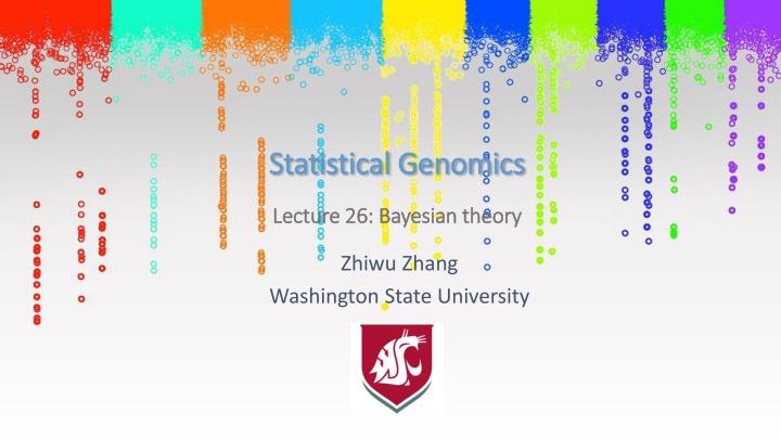
Statistical Genomics Statistical Genomics Lecture 26: Bayesian theory Lecture 26: Bayesian theory Zhiwu Zhang Washington State University
Outline Concept development for genomic selection Bayesian theorem Bayesian transformation Bayesian likelihood Bayesian alphabet for genomic selection
All SNPs have same distribution Ridge Regression gi~N(0, I g2) y=x1g1 + x2g2+ + xpgp + e K a2) gBLUP ~N(0, U
Selection of priors Out of control and overfitting! density.default(x = x) Flat Flat Identical normal 0.4 Density Problems of RR? 0.2 g2 0.0 g1 gp -4 -2 0 2 4 N = 10000 Bandwidth = 0.143 LSE RR solve LL solely solve REML by EMMA Distributions of gi
More realistic Out of control and overfitting? N(0, I gp2) N(0, I g12) N(0, I g22) y=x1g1 + x2g2+ + xpgp + e
Need help from Thomas Bayes "An Essay towards solving a Problem in the Doctrine of Chances" which was read to the Royal Society in 1763 after Bayes' death by Richard Price
An example from middle school A school by 60% boys and 40% girls. All boy wear pants. Half girls wear pants and half wear skirt. What is the probability to meet a student with pants? P(Pants) = 60%*100% + 40%*50% = 80%
Probability P(Pants) = 60%*100% + 40%*50% = 80% P(Boy)*P(Pants | Boy) + P(Girl)*P(Pants | Girl)
Inverse question A school by 60% boys and 40% girls. All boy wear pants. Half girls wear pants and half wear skirt. Meet a student with pants. What is the probability the student is a boy? P(Boy | Pants) 60%*100% = 75% 60%*100% + 40%*50%
P(Boy|Pants) 60%*100% = 75% 60%*100% + 40%*50% P(Pants | Boy) P(Boy) P(Pants | Boy) P(Boy) + P(Pants | Girl) P(Girl) P(Pants | Boy) P(Boy) P(Pants)
Bayesian theorem (parameters) P(Boy|Pants)P(Pants)=P(Pants|Boy)P(Boy) X Constant y(data)
Bayesian transformation Posterior distribution of given y (parameters) y(data) P( | y) P(Boy | Pants) P(Pants | Boy) P(Boy) Distribution of parameters (prior) P( ) Likelihood of data given parameters P(y| )
Bayesian for hard problem A public school containing 60% males and 40% females. What is the probability to draw four males? -- Probability (0.6^4=12.96%) Four males were draw from a public school. What are the male proportion? -- Inverse probability (?)
Prior knowledge density.default(x = x) Gender distribution density.default(x = x) density.default(x = x) 0.4 0.08 0.08 Density Density Density female 100% 100% male 0.2 0.04 0.04 0.00 0.00 0.0 0 10 20 30 40 -4 -2 0 2 4 40 30 20 10 0 N = 10000 Bandwidth = 0.6272 Likely N = 10000 Bandwidth = 0.143 N = 10000 Bandwidth = 0.6272 Safe unlikely Unsure Reject Four males were draw from a public school. What is the male proportion? -- Inverse probability (?)
Transform hard problem to easy one P(G|y) P(y|G) P(G) Probability of unknown given data (hard to solve) Probability of observed given unknown (easy to solve) Prior knowledge of unknown (freedom)
P(y|G) Probability of having 4 males given male proportion p=seq(0, 1, .01) n=4 k=n pyp=dbinom(k,n,p) theMax=pyp==max(pyp) pMax=p[theMax] plot(p,pyp,type="b",main=paste("Data=", pMax,sep="")) Data=1 0.8 pyp 0.4 0.0 0.0 0.2 0.4 0.6 0.8 1.0 Prior=0.5 p 0.4 0.3 0.2 pd 0.1 0.0 0.0 0.2 0.4 0.6 0.8 1.0 Optimum=0.57 0.030 ppy 0.015 0.000 0.0 0.2 0.4 0.6 0.8 1.0
P(G) Probability of male proportion (Prior) Data=1 ps=p*10-9 pd=dnorm(ps) theMax=pd==max(pd) pMax=p[theMax] plot(p,pd,type="b",main=paste("Prior=", pMax,sep="")) 0.4 0.8 pyp 0.0 0.0 0.2 0.4 0.6 0.8 1.0 Prior=0.5 0.4 0.3 0.2 pd 0.1 0.0 0.0 0.2 0.4 0.6 0.8 1.0 Optimum=0.57 0.030 ppy 0.015 0.000 0.0 0.2 0.4 0.6 0.8 1.0
Data=1 0.8 pyp 0.4 0.0 P(G|y) P(y|G) P(G) Prior=0.5 0.0 0.2 0.4 0.6 0.8 1.0 0.4 Probability of male proportion given 4 males drawn 0.3 0.2 pd ppy=pd*pyp theMax=ppy==max(ppy) pMax=p[theMax] plot(p,ppy,type="b",main=paste("Optimum=", pMax,sep="")) 0.0 0.2 0.1 0.0 0.4 0.6 0.8 1.0 Optimum=0.57 0.030 ppy 0.015 0.000 0.0 0.2 0.4 0.6 0.8 1.0
Depend what you believe Male=Female Much more male More Male Data=1 Data=1 Data=1 0.8 0.8 0.8 pyp pyp pyp 0.4 0.4 0.4 0.0 0.0 0.0 0.0 0.2 0.4 0.6 0.8 1.0 0.0 0.2 0.4 0.6 0.8 1.0 0.0 0.2 0.4 0.6 0.8 1.0 Prior=0.5 Prior=0.5 p Prior=0.7 0.4 0.4 0.4 0.3 0.3 0.3 0.2 0.2 pd 0.2 pd pd 0.1 0.1 0.1 0.0 0.0 0.0 0.0 0.2 0.4 0.6 0.8 1.0 0.0 0.2 0.4 0.6 0.8 1.0 0.0 0.2 0.4 0.6 0.8 1.0 Optimum=0.57 Optimum=0.57 Optimum=0.75 0.030 0.030 0.08 ppy 0.015 ppy ppy 0.015 0.04 0.000 0.000 0.00 0.0 0.2 0.4 0.6 0.8 1.0 0.0 0.2 0.4 0.6 0.8 1.0 0.0 0.2 0.4 0.6 0.8 1.0
Ten are all males More Male Male=Female Much more male Data=1 Data=1 Data=1 0.8 0.8 0.8 pyp pyp pyp 0.4 0.4 0.4 0.0 0.0 0.0 0.0 0.2 0.4 0.6 0.8 1.0 0.0 0.2 0.4 0.6 0.8 1.0 0.0 0.2 0.4 0.6 0.8 1.0 Prior=0.5 Prior=0.7 Prior=0.9 0.4 0.4 0.4 0.3 0.3 0.3 0.2 0.2 0.2 pd pd pd 0.1 0.1 0.1 0.0 0.0 0.0 0.0 0.2 0.4 0.6 0.8 1.0 0.0 0.2 0.4 0.6 0.8 1.0 0.0 0.2 0.4 0.6 0.8 1.0 Optimum=0.65 Optimum=0.82 Optimum=1 0.20 0.020 0.0010 vs. 57% vs. 75% vs. 94% ppy ppy ppy 0.10 0.010 0.0000 0.000 0.00 0.0 0.2 0.4 0.6 0.8 1.0 0.0 0.2 0.4 0.6 0.8 1.0 0.0 0.2 0.4 0.6 0.8 1.0
Bayesian transformation (likelihood) Posterior distribution of given y (parameters) y(data) P( | y) P(Boy | Pants) P(Pants | Boy) P(Boy) Distribution of parameters (prior) P( ) Likelihood of data given parameters P(y| )
More realistic Out of control and overfitting? Believe: Prior distributions N(0, I gp2) N(0, I g12) N(0, I g22) y=x1g1 + x2g2+ + xpgp + e
Outline Concept development for genomic selection Bayesian theorem Bayesian transformation Bayesian likelihood Bayesian alphabet for genomic selection


")


")
")


")