Introduction to Bayes' Rule: Understanding Probabilistic Inference

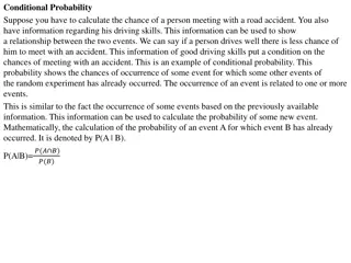
An overview of Bayes' rule, a fundamental concept in probabilistic inference, is presented in this text. It explains how to calculate conditional probabilities, likelihoods, priors, and posterior probabilities using Bayes' rule through examples like determining the likelihood of rain based on a wet lawn or the chance of the sprinkler being left on given wet grass. The text showcases the application of Bayes' rule in real-world scenarios to make informed decisions based on observed evidence.

• Bayes Rule
• Probabilistic Inference
• Conditional Probabilities
• Likelihood
• Posterior Probabilities

gwy_ke Follow

Uploaded on Sep 25, 2024 | 0 Views

Download Presentation

Please find below an Image/Link to download the presentation.

The content on the website is provided AS IS for your information and personal use only. It may not be sold, licensed, or shared on other websites without obtaining consent from the author. Download presentation by click this link. If you encounter any issues during the download, it is possible that the publisher has removed the file from their server.

Presentation Transcript

1. Bayes for beginners Claire Berna Lieke de Boer Methods for dummies 27 February 2013

2. Bayes rule Given marginal probabilities p(A), p(B), and the joint probability p(A,B), we can write the conditional probabilities: p(A,B) p(B|A) = p(A) p(A,B) p(A|B) = p(B) This is known as the product rule. p(A|B) p(B) Eliminating p(A,B) gives Bayes rule: p(B/A) = p(A)

3. Example: The lawn is wet : we assume that the lawn is wet because it has rained overnight: How likely is it? p(w|r) : Likelihood p(w|r) p(r) p(r|w) = p(w) What is the probability that it has rained overnight given this observation? p(r|w): Posterior: How probable is our hypothesis given the observed evidence? P(r): Prior: Probability to rain on that day. How probable was our hypothesis before observing the evidence? p(w) : Marginal: how probable is the new evidence under all possible hypotheses?

4. Example: p(w|r) p(r) p(r|w) = p(w) p(w=1|r=1) p(r=1) p(r=1|w=1) = p(w=1) The probability p(w) is a normalisation term and can be found by marginalisation. p(w=1) = p(w=1, r) r = p(w=1,r=0) + p(w=1,r=1) = p(w=1|r=0)p(r=0) + p(w=1|r=1)p(r=1) p(w=1 | r=1) = 0.95 p(w=1 | r=0) = 0.20 p(r = 1) = 0.01 This is known as the sum rule p(w=1|r=1) p(r=1) = 0.046 p(r=1|w=1) = p(w=1|r=0)p(r=0) + p(w=1|r=1)p(r=1)

5. Did I Leave The Sprinkler On ? A single observation with multiple potential causes (not mutually exclusive). Both rain, r , and the sprinkler, s, can cause my lawn to be wet, w. p(w, r , s) = p(r )p(s)p(w|r,s) Generative model

6. Did I Leave The Sprinkler On ? The probability that the sprinkler was on given i ve seen the lawn is wet is given by Bayes rule p(w=1|s=1) p(s=1) p(s=1|w=1) = p(w=1) p(w=1|s=1) p(s=1) = p(w = 1, s = 1) + p(w = 1, s = 0) where the joint probabilities are obtained from marginalisation and from the generative model: p(w, r , s) = p(r ) p(s) p(w|r,s) p(w = 1, s = 1) = 1 p(w = 1, r , s = 1) = p(w=1, r=0, s=1) + p(w=1, r=1, s=1) r=0 = p(r=0) p(s=1) p(w=1|r=0, s=1) + p(r=1) p(s=1) p(w=1|r=1, s=1) p(w = 1, s = 0) = 1 p(w = 1,r , s = 0) = p(w=1, r=0, s=0) + p(w=1, r=1, s=0) r=0 = p(r=0) p(s=0) p(w=1|r=0, s=0) + p(r=1) p(s=0) p(w=1|r=1, s=0)

7. Numerical Example Bayesian models force us to be explicit about exactly what it is we believe. p(r = 1) = 0.01 p(s = 1) = 0.02 p(w = 1|r = 0, s = 0) = 0.001 p(w = 1|r = 0, s = 1) = 0.97 p(w = 1|r = 1, s = 0) = 0.90 p(w = 1|r = 1, s = 1) = 0.99 These numbers give p(s = 1|w = 1) = 0.67 p(r = 1|w = 1) = 0.31

8. Look next door Rain r will make my lawn wet w1 and nextdoors w2 whereas the sprinkler s only affects mine. p(w1, w2, r, s) = p(r ) p(s) p(w1|r,s) p(w2|r )

9. After looking next door Use Bayes rule again p(w1=1, w2=1, s=1) p(s=1|w1=1, w2=1) = p(w1 = 1, w2 = 1, s = 1) + p(w1 = 1, w2 = 1, s = 0) with joint probabilities from marginalisation p(w1 = 1, w2 = 1, s = 1) = 1 p(w1 = 1, w2 = 1, r , s = 1) r=0 p(w1 = 1, w2 = 1, s = 0) = 1 p(w1 = 1;w2 = 1; r ; s = 0) r=0

10. Explaining Away Numbers same as before. In addition p(w2 = 1|r = 1) = 0.90 Now we have p(s = 1|w1 = 1, w2 = 1) = 0.21 p(r = 1|w1 = 1, w2 = 1) = 0.80 The fact that my grass is wet has been explained away by the rain (and the observation of my neighbours wet lawn).

11. The CHILD network Probabilistic graphical model for newborn babies with congenital heart disease Decision making aid piloted at Great Ormond Street hospital (Spiegelhalter et al. 1993).

12. Bayesian inference in neuroimaging When comparing two models A > B ? When assessing the inactivity of a brain area P(H0)

13. Assessing inactivity of brain area H0: = 0 define the null, e.g.: invert model (obtain posterior pdf) ( ) ( ) p t H p y 0 ( ) ( ) P H y * P t t H 0 0 ( ) t Y t t* H0: 0 estimate parameters (obtain test stat.) define the null, e.g.: apply decision rule, i.e.: apply decision rule, i.e.: ( ) ( ) * P t t H P H y if then reject H0 if then accept H0 0 0 classical approach Bayesian PPM

14. Bayesian paradigm likelihood function GLM: y = f( ) + From the assumption: noise is small Create a likelihood function with a fixed :

15. So needs to be fixed... priors Probability of , depends on: model you want to compare data previous experience Likelihood: Prior: Bayes' rule:

16. Bayesian inference Precision = 1/variance

17. Bayesian inference forward/inverse problem likelihood p(y| ) p( |y) posterior distribution

18. Bayesian inference Occam's razor The hypothesis that makes the fewest assumptions should be selected Plurality should not be assumed without necessity

19. Bayesian inference Hierarchical models hierarchy causality

20. References: - Will Penny s course on Bayesian Inference, FIL, 2013 http://www.fil.ion.ucl.ac.uk/~wpenny/bayes-inf/ - J. Pearl (1988) Probabilistic reasoning in intelligent systems. San Mateo, CA. Morgan Kaufmann. - Previous MfD presentations - Jean Daunizeau s SPM course a the FIL Thanks to Ged for his feedback!