Bayes Rule and Its Historical Significance
Bayes Rule, a fundamental theorem in statistics, helps in updating probabilities based on new information. This rule involves reallocating credibility between possible states given prior knowledge and new data. The theorem was posthumously published by Thomas Bayes and has had a profound impact on statistical inference. Pierre-Simon Laplace further developed the Bayesian approach, laying the foundation for probabilistic reasoning. The historical significance of Bayes Rule and its evolution contribute to modern scientific determinism and statistical methodologies like Bayesian inference.
Download Presentation

Please find below an Image/Link to download the presentation.
The content on the website is provided AS IS for your information and personal use only. It may not be sold, licensed, or shared on other websites without obtaining consent from the author.If you encounter any issues during the download, it is possible that the publisher has removed the file from their server.
You are allowed to download the files provided on this website for personal or commercial use, subject to the condition that they are used lawfully. All files are the property of their respective owners.
The content on the website is provided AS IS for your information and personal use only. It may not be sold, licensed, or shared on other websites without obtaining consent from the author.
E N D
Presentation Transcript
Bayes Rule Chapter 5 of Kruschke text Darrell A. Worthy Texas A&M University
Bayes rule On a typical day at your location, what is the probability that it is cloudy? Suppose you are told it is raining, now what is the probability that it is cloudy? Notice that those probabilities are not equal, because we can be pretty sure that p(cloudy) < p(cloudy|raining). Suppose instead you are told that everyone is wearing sunglasses. Now most likely p(cloudy) > p(cloudy|sunglasses).
Bayes rule Notice how we have reasoned in this example We started with the prior credibility allocated over two possible states of the sky: cloudy or sunny Then we took into account some other data; that it is raining or people are wearing sunglasses. Conditional on the new data, we reallocated credibility across the states of the sky. Bayes rule is merely the mathematical relation between the prior allocation of credibility and the posterior reallocation of credibility, given the data.
Historical Interlude Thomas Bayes (1702-1761) was a mathematician and Presbyterian minister in England. His famous theorem was only published posthumously thanks to his friend, Richard Price (Bayes & Price, 1763). The simple rule has vast ramifications for statistical inference. Bayes may not have fully comprehended the ramifications of his rule, however. Many historians have argued that it should be Laplace s rule, after Pierre-Simon Laplace (1749-1827).
Historical Interlude Laplace was one of the greatest scientists of all time. He was a polymath, studying physics and astronomy, in addition to developing calculus and probability theory. Laplace set out a mathematical system of inductive reasoning based on probability that is recognized today as Bayesian. This was done over a thirty year period where he developed the method of least squares used in regression and proved the first general central limit theorem. He showed that central limit theorem provided a Bayesian justification for the least squares method. In a later paper he used a non-Bayesian approach to show that ordinary least squares is the best linear unbiased estimator (BLUE).
Historical Interlude Bayesian, probabilistic reasoning is reflected in an 1814 treatise which included the first articulation of scientific determinism. In it is described Laplace s Demon , although he called it an intellect. We may regard the present state of the universe as the effect of its past and the cause of its future. An intellect which at a certain moment would know all forces that set nature in motion, and all positions of all items of which nature is composed, if this intellect were also vast enough to submit these data to analysis it would embrace in a single formula the movements of the greatest bodies of the universe and those to the tiniest atom; for such an intellect nothing would be uncertain and the future just like the past would be present before its eyes.
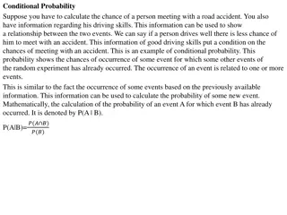
Conditional probability We often want to know the probability of one outcome, given that we know another outcome is true. Below are the probabilities for eye and hair color in the population. Suppose I randomly sample one person and tell you that they have blue eyes. Conditional on that information, what is the probability the person has blond hair given these data from the population?
Conditional probability This table shows the total (marginal) proportion of blue eyed people is .36 and the proportion of blue-eyed and blond-haired people is .16. Therefore, of the 36% with blue eyes .16/.36, or 45% have blond hair. We also know that there is a .39 probability that this blue eyed- person has brown hair.
Conditional Probability If we look back at our table of marginal and joint probabilities we can see that there is only a .21 probability of a person having blond hair. When we learn that this person has blue eyes, however, the probability of blond hair jumps to .45. This reallocation of credibility is Bayesian inference!
Conditional probability These intuitive computations for conditional probability can be denoted by simple formal expressions. The conditional probability of hair color given eye color is p(h|e); the | symbol reads as given This can be rewritten as p(h|e) = p(e,h)/p(e). The comma indicates a joint probability of a specific combination of eye and hair color, while p(e) is the marginal probability for a certain eye color. This equation is the definition of conditional probability. In Bayesian inference the end result is the conditional probability of a theory or parameter, given the data.
Conditional probability It s important to note that p(h|e) is not the same as p(e|h) For example, the probability that the ground is wet, given that it s raining is different than the probability that it s raining given that the ground is wet (the former is probably more likely than the latter). It s also important to note that there is no temporal order in conditional probabilities. When we say the probability of x given y it does not mean that y has already happened or that x has yet to happen. Another way to think of p(x|y) is, among all joint outcomes with value y, this proportion of them also has value x.
Bayes Rule Bayes rule is derived from the definition of conditional probability we just discussed. ? ? =?(?, ) ?(?) On page 100 of the Kruschke text it s shown that the above equation can be transformed into Bayes rule, which is: ? ? ?( ) ? ? ?( ) In the equation h in the numerator is a specified fixed value, and h* takes on all possible values. The transformations done to the numerator allow us to apply Bayes rule in powerful ways to data analysis ? ? =
Bayes Rule In the example involving eye and hair color joint probabilities p(e,h) were directly provided as numerical values. In contrast, Bayes rule involves joint probabilities expressed as p(e|h)*p(h). Expressing joint probabilities in this way was the main breakthrough that Bayes (and Laplace) had as it allowed for many statistical problems to be worked out. The next example provides a situation where it is natural to joint express probabilities as p(x|y)*p(y).
Bayes Rule Suppose you are trying to diagnose a rare disease. The probability of having this disease is 1/1000 We denote the true presence or absence of the disease as the value of parameter, , that can have a value of + or The base rate, p( = +)=.001, is our prior belief that a person selected at random has the disease. The test for the disease has a 99% hit rate, which means that if someone has the disease then the result is positive 99% of the time. The test also has a false alarm rate of 5%
Bayes Rule Suppose we sample at random from the population, administer the test, and it s positive. What, do you think, is the posterior probability that the person has the disease? Many people might say 99% since that is the hit rate of the test, but this ignores the extremely low base rate of the disease (the prior). As a side note, this could be analogous to a psychologist saying that the t-test is right 95% of the time, without taking into account the prior credibility of their (highly counter-intuitive) conclusions.
Bayes Rule The table below shows the joint probabilities of test results and disease states computed from the numerator of Bayes rule. The upper left corner shows us how to compute the joint probability that the test is positive and the disease is indeed present (.99 * .001) = .00099. But this is only the numerator of Bayes rule, to find the probability that a randomly chosen person has the disease, given a positive test we must divide by the marginal probability of a positive test.
Bayes Rule We know the test is positive so we look at the marginal likelihood of a positive test result (far right column). If the person has the disease then p(+| ) =.99 and the baseline likelihood of having the disease is .001. If they don t have the disease then p(+| ) = .05, and there is a .999 probability within the population. The denominator then is .99*.001+.05*.999 = .0509
Bayes Rule Taking the joint probability (.00099) of the person testing positive and also having the disease, and dividing that by the marginal probability of receiving a positive test (.05094) yields a conditional probability that this person actually has the disease, given the positive test, of .019. Yes, that s correct. Even with a positive test result with a hit rate of 99% the posterior probability of having the disease is only .019. This is due to the low prior probability of having the disease and a non-negligible false alarm rate (5%). One caveat is that we took the person at random if they had other symptoms that motivated the test then we should take that into account.
Bayes Rule To summarize: we started with the prior credibility of the two disease states (present or absent) We used a diagnostic test that has a known hit and false alarm rate, which are the conditional probabilities of a positive test result, given each possible disease state. When an observed test result occurred we computed the conditional probabilities of disease states in that row using Bayes rule. The conditional probabilities are the re-allocated credibilities of the disease states, given the data.
Applied to Parameters and Data The key application that makes Bayes rule so useful is when the row variable in the table below represents data values (like the test result), and the column variable represents parameter values (what we want to infer like what values of Student s t are most probable, given our data). This gives us a model of data, given specific parameter values and allows us to evaluate evidence for that model from the data.
Applied to Parameters and Data A model of data specifies the probability of particular data values given the model s structure and parameter values. The model also indicates the probability of the various parameter values. In other words the model specifies p(data values | parameter values) along with prior, p(parameter values). We use Bayes rule to convert that to what we really want to know, which is how strongly we should believe in the various parameter values, given the data: p(parameter values | data values).
Applied to Parameters and Data The two-way table below can help thinking about how we are applying Bayes rule to parameters and data. The columns correspond to specific parameter values, and the rows specific values of data. Each cell holds the joint probability of the specific combination of parameter value, , and data value D.
Applied to Parameters and Data When we observe a particular data value, D, we restrict our attention to the specific row of this table that corresponds to value D. The prior probability of the parameter values is the marginal distribution, p( ), which is in the lower row. The posterior distribution on is obtained by dividing the joint probabilities in that row by the marginal probability, p(D).
Applied to Parameters and Data Bayes rule is shifting attention from the prior marginal distribution of the parameter values to the posterior, conditional distribution of parameter values for a specific value of data. The factors of Bayes rule have specific names. p( |D) = p(D| ) * p( ) / p(D) posterior likelihood prior evidence Evidence, the denominator can be rewritten as: ? ? ? ? ?(? ) Again, the asterisk indicates that we are referring to all possible parameter values rather than specific ones in the numerator.
Applied to Parameters and Data The prior, p( ), is the credibility of the parameter values without the data. The posterior, p( |D), is the credibility of the parameter values after taking the data into account. The likelihood, p(D| ), is the probability that the data could be generated with parameter value . The evidence for the model, p(D), is the overall probability of the data according to the model, determined by averaging across all possible parameter values weighted by the strength of belief in those parameter values.
Applied to Parameters and Data The denominator of Bayes rule, or evidence, is also called the marginal likelihood. So far we ve discussed Bayes rule in the context of discrete-valued variables (has the disease or not). It also applies to continuous variables, but probability masses become probability densities, and sums become integrals. For continuous variables, the only change is that the marginal likelihood changes from a sum to an integral: ? ? = ?? ? ? ? ?(? )
Estimating bias in a coin As an example of Bayesian analysis of continuous outcomes we will use Bayes rule to determine the bias, or underlying probability that the coin flips heads, from the data. Kruschke s text goes into more detail than I will present on the underlying math behind our operations. I will focus more on the results from different examples and how different types of data (number of coin flips and proportion that were heads) affect the likelihood and posterior.
Estimating bias in a coin Suppose we have a coin factory that tends to make fair coins, but they also tend to err a lot and make coins that are more or less likely to come up heads with repeated flips. represents the true value of the coin that we are trying to infer from the data. We consider 1001 possibilities for the true value of and construct a triangular prior where .5 is the most likely value, but other values are also possible.
Estimating bias in a coin Suppose we flipped the coin four times and only one of these four were heads. The prior, likelihood, and posterior are shown to the right. Note that the width of the 95% HDI is large and includes the value of .5.
Estimating bias in a coin Now suppose we still observed that 25% of the flips were heads, but from 40 observations. The posterior distribution is much narrower and .5 is no longer included in the 95% HDI. The posterior will be less influenced by the prior distribution as sample size increases.
Estimating bias in a coin In general broad priors have less effect on the posterior distribution than sharper, narrower priors. This plot shows the same data with N=40 and proportion of heads =.25. Due to the sharp prior around .5 the posterior is less influenced by the data.
Priors For most applications prior specification is technically unproblematic. We will use vague priors that do not give too much credit to unrealistic values (e.g. =5) Prior beliefs should influence rational inference from the data, and they should be based on publicly agreed upon facts or theories. This may be applicable to many counter-intuitive findings that have recently proven difficult to replicate. For example, perhaps our priors should reflect the fact that most people do not believe in ESP, and we will need strong evidence to overturn this prior belief.
Why Bayesian analysis can be difficult Because of this ? ? = ?? ? ? ? ?(? ) The integral form of the marginal likelihood function can be impossible to solve analytically. In the previous example with coin flips we used numerical approximation of the integral. This will not work, however, as the number of parameters to estimate increases (e.g. multiple regression coefficients). The space of possibilities is the joint parameter space. If we subdivide the possible parameter space into 1000 regions, as in the previous examples then we have 1000pparameter values.
Why Bayesian analysis can be difficult Markov Chain Monte Carlo (MCMC) methods are another approach. Here we sample a large number of representative combinations of parameter values from the posterior distribution. MCMC is so powerful because it can generate representative parameter-value combinations from the posterior distribution of very complex models without computing the integral in Bayes rule. This is by far the most common method currently used and what has allowed Bayesian statistical analyses to gain practical use over the past thirty years.
