Understanding Automated Theorem Proving in Lean
Dive into the world of automated theorem proving in Lean with a focus on formal verification, history, and the use of logic and computational methods. Explore how programs can assist in finding and verifying proofs, as well as the significance of interactive theorem provers. Discover the evolution of automated theorem proving and the various methods used to check formula validity in propositional and first-order logic.
Download Presentation

Please find below an Image/Link to download the presentation.
The content on the website is provided AS IS for your information and personal use only. It may not be sold, licensed, or shared on other websites without obtaining consent from the author. Download presentation by click this link. If you encounter any issues during the download, it is possible that the publisher has removed the file from their server.
E N D
Presentation Transcript
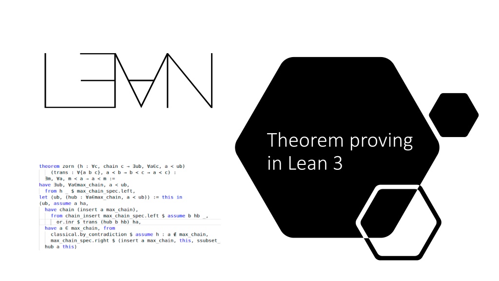
Theorem proving in Lean 3
What is covered in that presentation from Lean documentation 1. Introduction the whole chapter 2. Dependent Type Theory up to 2.7. Namespaces, without 2.8. Dependent Types, 2.9. Implicit Arguments and 2.10. Exercises
Introduction Terminology
Formal verification The use of logic and computational methods to check if the claim, written in a precise mathematical form, is true or false. Example of a claim: (A B) (B A) Verification: 1. A B 2. A B A 3. A B B 4. A 5. B 6. B (A B A) 7. A B A 8. B A (Resource of example: Y.Belov, V.Sokolov)
Two ways how we can make a program to provide a proof A program can find a proof A program can help verify that the given proof is correct
Automated theorem proving A theorem proving, where a proof is realized by computer program. The process of proving is based on propositional and first-order logic The process is searching powerful, efficient system can have bugs. Are the results correct?
History of automated theorem proving JOHNNIAC (1954, Martin Davis), proved that the sum of two even numbers is even Logic Theory Machine (1956, Allen Newell, Herbert A. Simon and J. C. Shaw) ran on JOHNNIAC, constructed proofs from a small set of propositional axioms and three deduction rules: modus ponens, (propositional) variable substitution, and the replacement of formulas by their definition. Managed to prove 38 of the first 52 theorems of the Principia JOHNNIAC, photo from http://ed-thelen.org
What can we do using ATP Check the validity of formulas in propositional and first-order logic: Resolution theorem provers Tableau theorem provers Fast satisfiability solvers Search and check the validity expression in specific languages or domains (e.g., of linear or nonlinear expressions over the integers or the real numbers) Realize mathematical computations, establish mathematical bounds, find mathematical objects. Calculation equals to proof here.
Interactive theorem prover A software, that assists the development of formal proofs A human guides the search for proofs. Computer provides and stores the details of proof The process is verifying every claim should be supported by a proof in a suitable axiomatic foundation more input and interaction from user allow to obtain deeper and more complex proof
Interactive theorem proving Resource: Tianxiang Lu on researchgate.net
The aim of Lean To bridge the gap between interactive and automated theorem proving It has automated tools and methods inside a framework User interacts with that framework and constructs axiomatic proofs
The goal of Lean To support both mathematical reasoning and reasoning about complex systems, and to verify claims in both domains Programmaticaly speaking, to prove things about the objects we define So, what can we verify in Lean: Ordinary mathematical theorems Claims about correctness of the programming code, hardware, software, network protocols, mechanical and hybrid systems...
Ordinary mathematical theorems, claims about correctness of programming code, hardware, software, network protocols, mechanical and hybrid systems... WHY ON THE SAME LEVEL SAME LEVEL?
CurryHoward isomorphism There is a direct relationship between computer programs and mathematical proofs: Hardware and software systems are described in mathematical terms, the check of its correctness is a theorem proving A theorem proof is basically computations, a program. The formula it proves is the type for the program Proofs can be represented as programs, proofs can be run
How Lean can be used? As a programming language, as a system for writing programs with a precise semantics and for reasoning about the functions that the programs compute As a metaprogramming language we can extend the functionality of Lean using the Lean itself
How to use Lean? In browser Install a program, which is faster and more flexible, than Lean in browser Lean in VIM editor (download e.g. VS Code if you are a Windows user) Resource: yakovlev.me
2. Dependent Type Theory
Dependent type theory Powerful, expressive Provides a natural and uniform expressions of complex mathematical assertions, hardware and software specifications Every term has a computational behavior (they can be computed) Lean is based on a version of dependent type theory Calculus of Constructions
Why to use type theory in provers? We can track various kinds of mathematical objects: natural numbers, functions on a natural numbers, booleans We can build new types
constant, constants to declare constants, which then available everywhere in code constant a : bool constants m n : nat variable, variables to declare constants, that are available inside a block of code (?? ask) section to define a block of code, can be nested (sections inside sections). Use it to declare variables for insertion in theorems. It is not necessary to give a name to section, but if you do, it is necessary to close it using the same name section useful variable x : --more computations here end useful namespace for grouping definitions, can be nested (namespaces inside namespaces). Use it to organize data. namespace foo def a : := 5 end foo -- we call it outside like `foo.a` def to define an object in a form def foo : := bar namespace foo def a : := 5 end foo -- we call it outside like `foo.a` def double : := x, x + x def double (x : ) : := x + x Lean commands universe to declare a universe variable universe u constant : Type u
Lean commands # - the beginning for commands #check to check the type of a constant or the type of operation #check ( x : , x) a #print to print something on a screen #print here I declare constants #reduce to evaluate an expression by reducing it to normal form (by carrying out all the computational reductions that are sanctioned by the underlying logic) constant n : nat #reduce n + 0 -- n #reduce n + 2 -- nat.succ (nat.succ n) #reduce 2 + 3 -- 5 #eval the other command to evaluate an expression, less trustworthy, more efficient -- comments, /- also comments -/ #check ( x : , x) a #print here I declare constants constant n : nat #reduce n + 0 -- n #reduce n + 2 -- nat.succ (nat.succ n) #reduce 2 + 3 -- 5
Typing helper To type type \to, \r or -> To type type nat or \nat To type type \times To type letters like , , and , type \a, \b, \g
Type In type theory, every expression has an associated type natural number, Boolean, function In Lean everything is a type. Types also have a type of Type, and Type has a type of Type in an infinite hierarchy of types. You can define your own types in Lean
Lets look at types in Lean closer 2 Declaring a universe type variable We declared new types and Types have a type of Type Declaring a type variable without creating a universe An infinite hierarchy of types lies in foundation of Lean: Type 0 (or Type) is a universe of "small" or "ordinary" types. Type 1 is a larger universe of types, which contains Type 0 as an element. Type 2 is a larger universe of types, which contains Type 1 as an element, etc.
Functions in Lean nat nat denotes the type of functions that take a natural number as input and return a natural number as output constant f : nat nat (m, n) denotes the ordered pair of m and n, and if p is a pair, p.1 and p.2 denote the two projections constants m n : nat constant p : nat nat #check p.1 -- #check (m, n) -- #check (p.1, n) -- The application of a function f to a value x is denoted f x #check f x -- When writing type expressions, arrows associate to the right; for example, in code constant g : nat nat nat, the type of g is nat (nat nat) g is a function that takes natural numbers and returns another function that takes a natural number and returns a natural number at the end, the number is returned This process is called currying constant f : nat nat constants m n : nat constantp : nat nat #check p.1 -- #check (m, n) -- #check (p.1, n) -- #check f x --
Creating a function from another expression We need a lambda abstraction process here (we need to turn terms and parts of terms into a variable) We temporarily postulate a variable x : , and then we can construct an expression t : The expression fun x : , t, or, equivalently, x : , t, is an object of type It is a function from to which maps any value x to the value t, which depends on x Let f be the function which maps any natural number x to x + 5 #check fun x : nat, x + 5 #check x : nat, x + 5
Some terminology Bound variable a placeholder with the given scope x : , t - x is a placeholder, whose "scope" doesn't extend beyond t Alpha equivalent expressions the expressions that are the same up to a renaming of bound variables, they are considered the same. (b : ) (x : ), x is equal to (u : ) (z : ), z Identity function a function that always returns the same value that was used as its argument Graph of the identity function on the real numbers, Resource: Wikipedia
Some terminology 2 Constant function a function whose (output) value is the same for every input value, e.g., f(x) = 4 is a constant function Function composition applying one function to the results of another
The expression x : , x denotes the identity function on , the expression x : , b denotes the constant function that always returns b, and x : , g (f x), denotes the composition of f and g Lean interprets the final three examples as the same expression; in the last expression, Lean infers the type of x and y from the types of f and h We can abstract over any of the constants in the previous definitions We can even abstract over the type The function that takes three types, , , and , and two functions, g : and f : , and returns the composition of g and f
#reduce #reduce Beta reduction - the process of simplifying an expression. E.g., simplifying ( x, t)s to t[s/x] - t with s substituted for the variable x Beta equivalent terms - terms that beta reduce to a common term Definitionally equal term two terms that reduce to the same value In dependent type theory every term has a computational behavior, and supports a notion of reduction, or normalization
How we are working in Lean most of the time? We define objects and prove things about them def double : := x, x + x def square : := x, x * x def do_twice : ( ) := f x, f (f x) def double (x : ) : := x + x def square (x : ) := x * x def do_twice (f : ) (x : ) : := f (f x) def do_twice ( : Type*) (h : ) (x : ) : := h (h x) def do_twice (h : ) (x : ) : := h (h x) variables ( : Type*) variables (g : ) (f : ) (h : ) variable x : def do_twice := h (h x)
Local definitions using let let a := t1 in t2 means all a in t2 will be replaced by t1 #reduce let y := 2 + 2, z := y + y in z * z -- 64 - all z are replaced by y + y, which are 4+4, so z * z equals to 64 def t (x : ) : := let y := x + x in y * y #reduce t 2 -- 16
Namespaces Like sections, nested namespaces have to be closed in the order they are opened Namespaces cannot be declared inside a section namespace foo def a : := 5 #print "inside foo" #check a end foo #print "outside the namespace" -- #check a -- error open foo #print "opened foo" #check a
Resources https://en.wikipedia.org/wiki/Curry%E2%80%93Howard_correspond ence https://yakovlev.me/lean-intro/ https://leanprover.github.io/theorem_proving_in_lean/ https://commons.wikimedia.org/w/index.php?curid=66273005 https://ru.wikipedia.org/wiki/%D0%90%D0%B2%D1%82%D0%BE%D0 %BC%D0%B0%D1%82%D0%B8%D1%87%D0%B5%D1%81%D0%BA%D 0%BE%D0%B5_%D0%B4%D0%BE%D0%BA%D0%B0%D0%B7%D0%B0 %D1%82%D0%B5%D0%BB%D1%8C%D1%81%D1%82%D0%B2%D0%B E#cite_note-1
