Time Series Model Estimation: Overview and Methods

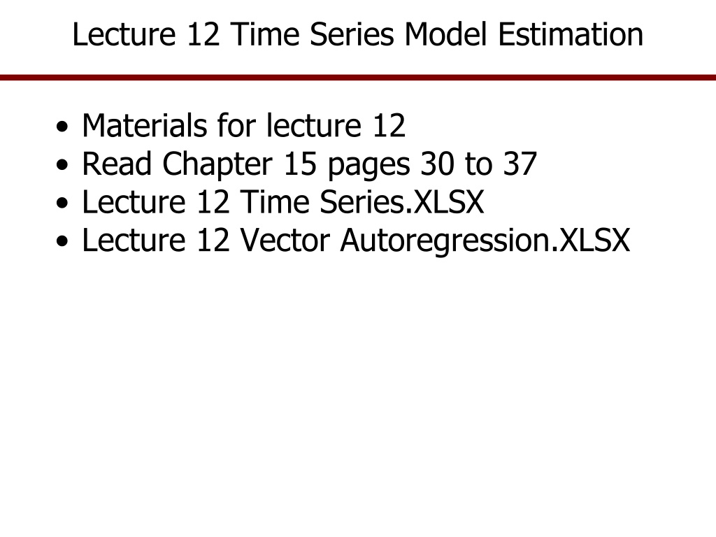
Lecture 12 Time Series Model Estimation Materials for lecture 12 Read Chapter 15 pages 30 to 37 Lecture 12 Time Series.XLSX Lecture 12 Vector Autoregression.XLSX

Time Series Model Estimation Outline for this lecture Review stationarity and no. of lags Discuss model estimation Demonstrate how to estimate Time Series (AR) models with Simetar Interpretation of model results How to forecast the results for an AR model

Time Series Model Estimation Plot the data to see what kind of series you are analyzing Make the series stationary by determining the optimal number of differences based on =DF() test, say Di,t Determine the number of lags to use in the AR model based on =AUTOCORR() or =ARLAG() Di,t=a + b1Di,t-1+ b2Di,t-2+b3Di,t-3+ b4Di,t-4 Create all of the data lags and estimate the model using OLS (or use Simetar)

Time Series Model Estimation An alternative to estimating the differences and lag variables by hand and using an OLS regression package, we will use Simetar Simetar time series function is driven by a menu

Time Series Model Estimation Read output as a regression output Beta coefficients are OLS slope coefficients SE of Coef. used to calculate t ratios to determine which lags are significant For goodness of fit refer to AIC, SIC and MAPE Can test restricting out lags (variables) AR Series Analysis Results for 2 Lags & 1 Difference, 2/27/2012 8:12:25 PM Constant SalesL1 SalesL2 Sales 3.393 0.476 S.E. of Coefficients Sales 30.764 0.144 Restriction Matrix Sales 1 1 Differences 1 Characteristics Dickey-Fuller Test Aug. Dickey-Fuller Test Schwarz S.D. Residuals Sales -4.471 -4.271 Forecast Impulse Auto- t-Statistic Partial ResponseCorrelation (AutoCorr.) AutoCorrelation -0.107 0.143 1 MAPE AIC SIC 5.529 212.955 8.86 10.84 10.95345 t-Statistic (Part.AutoCorr.) Period

Before You Estimate TS Model (Review) Dickey-Fuller test indicates whether the data series used for the model, Di,t, is stationary and if the model is D2,t= a + b1D1,tthe DF it indicates that t stat for b1is < -2.90 Augmented DF test indicates whether the data series Di,t are stationary, if we added a trend to the model and one or more lags Di,t=a + b1Di,t-1+ b2Di,t-2+b3Di,t-3+ b4Tt SIC indicates the value of the Schwarz Criteria for the number lags and differences used in estimation Change the number of lags and observe the SIC change AIC indicates the value of the Aikia information criteria for the number lags used in estimation Change the number of lags and observe the AIC change Best number of lags is where AIC is minimized Changing number of lags also changes the MAPE and SD residuals

Forecasting a Time Series Model If we assume a series that is stationary and has T observations of data we estimate the model as an AR(0 difference, 1 lag) Forecast the first period ahead as T+1= a + b1YT Forecast the second period ahead as T+2= a + b1 T+1 Continue in this fashion for more periods This ONLY works if Y is stationary, based on the DF test for zero lags

Forecasting a Times Series Model What if D1,twas stationary? How do you forecast? First period ahead forecast is Recall that D1,T = YT YT-1 So the regression lets us: D 1,T+1= a + b1D1,T Next add the forecasted D1,T+1to YT to forecast T+1 as follows: T+1= YT+ D 1,T+1

Forecasting A Time Series Model Second period ahead forecast is D 1,T+2= a + b D 1,T+1 T+2= T+1+ D 1,T+2 Repeat the process for period 3 and so on This is referred to as the chain rule of forecasting

For Forecast Model D1,t= 4.019 + 0.42859 D1,T-1 Year History and Forecast T+i 1387 Change or D 1,T Forecast D1T+i Forecast T+i T-1 T 1289 -98.0 -37.925 = 4.019 + 0.428*(-98) 1251.1 = 1289 + (-37.925) T+1 1251.1 -37.9 -12.224 = 4.019 + 0.428*(-37.9) -1.198 = 4.019 + 0.428*(-12.19) 1238.91 = 1251.11 + (-12.22) 1237.71=1238.91 + (-1.198) T+2 1238.91 -12.19 T+3 1237.71

Time Series Model Forecast AR Series Analysis Results for 2 Lags & 1 Difference, 2/27/2012 8:12:25 PM Constant SalesL1 SalesL2 Sales 3.028 0.430 S.E. of Coefficients Sales 30.621 0.129 Restriction Matrix Sales 1 1 Differences 1 Characteristics Dickey-Fuller Test Aug. Dickey-Fuller Test Schwarz S.D. Residuals Sales -4.471 -4.271 Forecast Impulse Auto- t-Statistic Partial ResponseCorrelation (AutoCorr.) AutoCorrelation 1,249.849 1.000 0.427042 3.108914 0.427042 3.108914 1,236.027 0.431 0.096647 0.602284 1,233.106 0.186 0.073858 0.457153 1,234.877 0.080 0.109992 0.678136 0.062501 0.455016 1,238.667 0.034 0.033193 0.202893 0.000 0.000 0 MAPE AIC 5.529 214.1866 9.06 10.81 t-Statistic (Part.AutoCorr.) Period 1 2 3 4 5 -0.10484 0.09031 0.657466 -0.76322 -0.05185 -0.37748

Time Series Model Estimation Impulse Response Function Shows the impact of a 1 unit change in YTon the forecast values of Y over time Good model is one where impacts decline to zero in short number of periods Impulse Response Function 1.200 1.000 0.800 0.600 0.400 0.200 0.000

Time Series Model Estimation Impulse Response Function will die slowly if the model has to many lags; they feed on themselves Same data series fit with 1 lag and a 6 lag model

Time Series Model Estimation Dynamic stochastic Simulation of a time series model Lecture 6

Time Series Model Estimation Look at the simulation in Lecture 12 Time Series.XLS

Time Series Model Estimation Result of a dynamic stochastic simulation

Vector Autoregressive (VAR) Models VAR models are time series models where two or more variables are thought to be correlated and together they explain more than one variable by itself For example forecasting Sales and Advertising Money supply and interest rate Supply and Price We are assuming that Yt = f(Yt-i and Zt-i)

VAR Time Series Model Estimation Take the example of advertising and sales AT+i = a +b1DA1,T-1 + b2 DA1,T-2 + c1DS1,T-1 + c2 DS1,T-2 ST+i = a +b1DS1,T-1 + b2 DS1,T-2 + c1DA1,T-1 + c2 DA1,T-2 Where A is advertising and S is sales DA is the difference for A DS is the difference for S In this model we fit A and S at the same time and A is affected by its lag differences and the lagged differences for S The same is true for S affected by its own lags and those of A

Time Series Model Estimation Advertising and sales VAR model Highlight two columns Specify number of lags Specify number differences

Time Series Model Estimation Advertising and sales VAR model