Statistical Inference and Estimation in Probabilistic System Analysis
This content discusses statistical inference methods like classical and Bayesian approaches for making generalizations about populations. It covers estimation problems, hypothesis testing, unbiased estimators, and efficient estimation methods in the context of probabilistic system analysis. Examples include estimating voter preferences and testing product quality. Dr. Erwin Sitompul from President University provides valuable insights in this lecture series.

Download Presentation

Please find below an Image/Link to download the presentation.
The content on the website is provided AS IS for your information and personal use only. It may not be sold, licensed, or shared on other websites without obtaining consent from the author.If you encounter any issues during the download, it is possible that the publisher has removed the file from their server.
You are allowed to download the files provided on this website for personal or commercial use, subject to the condition that they are used lawfully. All files are the property of their respective owners.
The content on the website is provided AS IS for your information and personal use only. It may not be sold, licensed, or shared on other websites without obtaining consent from the author.
E N D
Presentation Transcript
Probabilistic System Analysis Lecture 12 Dr.-Ing. Erwin Sitompul President University http://zitompul.wordpress.com 2 0 2 2 President University Erwin Sitompul PSA 12/1
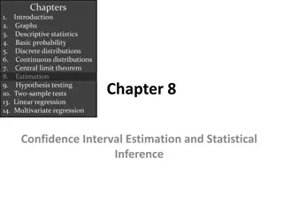
Chapter 9 One- and Two-Sample Estimation Problems Chapter 9 One- and Two-Sample Estimation Problem President University Erwin Sitompul PSA 12/2
Chapter 9.2 Statistical Inference Statistical Inference The theory of statistical inference consists of those methods by which one makes inferences or generalizations about a population. The methods are distinguished by: Classical Method, estimating a population parameter based strictly on information obtained from a random sample selected from the population. Bayesian Method, estimating a population parameter by utilizing prior subjective knowledge about the probability distribution of the unknown parameters in conjunction with the information provided by the sample data. President University Erwin Sitompul PSA 12/3
Chapter 9.2 Statistical Inference Areas of Statistical Inference Estimation, a random sample is taken from the population, then the statistic of the sample is used to estimate the statistic of the population. A candidate for public office may wish to estimate the true proportion of voters favoring him by obtaining the opinions from a random sample of 100 eligible voters. Test of Hypotheses, a hypothesis about a population is stated and a random sample is taken from the population, then the statistic of the sample is used to test the hypothesis and finally come to a correct decision to accept or reject it. Someone is interested in finding out whether brand A floor wax is more scuff-resistant than brand B floor wax. The hypothesis is that brand A is better than brand B. After some tests, he can decide to accept or reject this hypothesis. President University Erwin Sitompul PSA 12/4
Chapter 9.3 Classical Methods of Estimation Classical Methods of Estimation A point estimate of some population parameter is a single value of a statistic . For example, the value x of the statistic X, computed from a sample of size n, is a point estimate of the population parameter . ^ ^ _ _ An estimator is not expected to estimate the population parameter without error. We do not expect X to estimate exactly, but we certainly hope that it is not far off. We would always choose an estimator that has a mean equal to the parameter estimated. An estimator possessing this property is said to be unbiased. _ ^ ^ A statistic is said to be an unbiased estimator of the parameter if ( ) = E = President University Erwin Sitompul PSA 12/5
Chapter 9.3 Classical Methods of Estimation Classical Methods of Estimation If we consider all possible unbiased estimators of some parameter , the one with the smallest variance is called the most efficient estimator of . ^ The most efficient estimator is 1 Which one is more efficient between 2 and 3? ^ ^ President University Erwin Sitompul PSA 12/6
Chapter 9.3 Classical Methods of Estimation Interval Estimation Even the most efficient unbiased estimate is unlikely to estimate the population parameter exactly. It is unlikely that a point estimate from a given sample will be exactly equal to the population parameter it is supposed to estimate. So, there are many situations in which it is preferable to determine an interval within which we would expect to find the value of the parameter. Such an interval is called an interval estimation. An interval estimate of a population parameter is an interval of the form , where and depend on the value of the statistic for a particular sample and also on the sampling distribution of . L U L U President University Erwin Sitompul PSA 12/7
Chapter 9.3 Classical Methods of Estimation Interpretation of Interval Estimates If, for instance, we find and such that ( ) 1 = L U P U L for 0 < < 1, then we have a probability of 1 of selecting a random sample that will produce an interval containing . The interval , computed from the selected sample, is then called a (1 )100% confidence interval. The fraction 1 is called the confidence coefficient or the degree of confidence. The endpoints are called the lower and upper confidence limits. L U and L U President University Erwin Sitompul PSA 12/8
Chapter 9.3 Classical Methods of Estimation Interpretation of Interval Estimate Thus, when = 0.05, we have a 95% confidence interval, when = 0.01, we obtain a wider 99% confidence interval. The wider the confidence interval is, the more confident we can be that the given interval contains the unknown parameter. Degree of confidence must be so chosen that the data is useful for further application. For example, it is better to be 95% confident that the average life of a certain television transistor is between 6 and 7 years than to be 99% confident that it is between 3 and 10 years. President University Erwin Sitompul PSA 12/9
Chapter 9.4 Single Sample: Estimating the Mean Single Sample: Estimating the Mean We already found out previously, that x is likely to be a very accurate estimate of when n is large. Let us now consider the interval estimate of . If the sample is selected from a normal population or if n is sufficiently large, we can establish a confidence interval for by considering the sampling distribution of X. _ _ President University Erwin Sitompul PSA 12/10
Chapter 9.4 Single Sample: Estimating the Mean Estimating the Mean (known ) According to the Central Limit Theorem, we can expect the sampling distribution of X to be approximately normally distributed with mean and standard deviation given by = = n and X X Writing z /2 for the z-value above which we find an area of /2, we can see from the figure below, that ( 2 2 1 P z Z z = X Z n ) = where X = 1 P z z 2 2 n + = 1 P X z X z 2 2 n n President University Erwin Sitompul PSA 12/11
Chapter 9.4 Single Sample: Estimating the Mean Estimating the Mean (known ) We now calculate the (1 )100% confidence interval of the mean of a random sample of size n selected from a population whose variance 2 is known by the resulting formula. _ If x is the mean of a random sample of size n from a population with known variance 2, a (1 )100% confidence interval for is given by + x z x z 2 2 n n where z /2 is the z-value leaving an area of /2 to the right. The case of known + z x z 2 2 n n President University Erwin Sitompul PSA 12/12
Chapter 9.4 Single Sample: Estimating the Mean Estimating the Mean (known ) Different samples will yield different value of x and therefore produce different interval estimates of the parameter , as shown below. _ The circular dots at the center of each interval indicate the position of the point estimate x for each random sample. Most of the intervals are seen to contain , but not in every case. _ The larger the value we choose for z /2, the wider we make all the intervals and the more confident we can be that the particular sample selected will produce an interval that contains the unknown parameter . But, larger range can also means larger deviation of x from . _ + x z x z 2 2 n n + z x z 2 2 n n President University Erwin Sitompul PSA 12/13
Chapter 9.4 Single Sample: Estimating the Mean Estimating the Mean (known ) The average zinc concentration recovered from a sample of zinc measurements in 36 different locations is found to be 2.6 g/ml. Find the 95% and 99% confidence intervals for the mean zinc concentration in the river. Assume that the population standard deviation is 0.3. = = 2.6, 0.3 x = 1.96 z 0.025 0.3 36 0.3 36 2.6 (1.96) 2.6 (1.96) + Degree of confidence 95% 2.5 2.70 = 2.575 z 0.005 0.3 36 0.3 36 2.6 (2.575) 2.6 (2.575) + Degree of confidence 99% 2.47 2.73 President University Erwin Sitompul PSA 12/14
Chapter 9.4 Single Sample: Estimating the Mean Estimating the Mean (known ) We can be (1 )100% sure that the error will not exceed President University Erwin Sitompul PSA 12/15
Chapter 9.4 Single Sample: Estimating the Mean Estimating the Mean (known ) President University Erwin Sitompul PSA 12/16
Chapter 9.4 Single Sample: Estimating the Mean Estimating the Mean (known ) How large a sample is required in the previous example, if we want to be 95% confident that our estimate of is off by less than 0.05? = 0.3 2 (1.96)(0.3) 0.05 Therefore, we can be 95% confident that a random sample of size 139 will provide an estimate x differing from by an amount less than 0.05. = = 138.3 n _ President University Erwin Sitompul PSA 12/17
Chapter 9.4 Single Sample: Estimating the Mean One-Sided Confidence Bounds The confidence intervals and resulting confidence bounds discussed this far are two sided (both upper and lower bounds are given). However, there are many applications in which only one bound is of interest. When measuring the mercury composition in a river, we only need to know, that for a certain degree of confidence, the level is below a certain upper bound. President University Erwin Sitompul PSA 12/18
Chapter 9.4 Single Sample: Estimating the Mean One-Sided Confidence Bounds President University Erwin Sitompul PSA 12/19
Chapter 9.4 Single Sample: Estimating the Mean Estimating the Mean (unknown ) Frequently, we attempt to estimate the mean of a population when the variance is unknown. We should recall that in previous chapter we learned that if we have a random sample from a normal distribution, then the random variable X T S n = has a Student s t-distribution with n 1 degrees of freedom, where S is the sample standard deviation. In this case with unknown, T can be used to construct a confidence interval on . The procedure is the same except is replaced by S and the standard normal distribution is replaced by the t-distribution. President University Erwin Sitompul PSA 12/20
Chapter 9.4 Single Sample: Estimating the Mean Estimating the Mean (unknown ) Referring to the next figure, we can assert that ( 2 2 1 P t T t = ) n X S = 1 P t t 2 2 S S + = 1 P X t X t 2 2 n n The case of unknown President University Erwin Sitompul PSA 12/21
Chapter 9.4 Single Sample: Estimating the Mean Estimating the Mean (unknown ) The case of unknown President University Erwin Sitompul PSA 12/22
Chapter 9.4 Single Sample: Estimating the Mean t-Distribution Table President University Erwin Sitompul PSA 12/23
Chapter 9.4 Single Sample: Estimating the Mean Estimating the Mean (unknown ) The contents of 7 similar containers of sulfuric acid are 9.8, 10.2, 10.4, 9.8, 10.0, 10.2, and 9.6 liters. Find a 95% confidence interval for the man of all such containers, assuming an approximate normal distribution. x = s = 10.0 0.283 Using the t-Distribution Table, we find that t0.025 = 2.447 for v = 6. Hence, the 95% confidence interval for is s s x t x t n n 0.283 10.0 (2.447) 10.0 (2.447) 7 + 2 2 0.283 + 7 9.74 10.26 President University Erwin Sitompul PSA 12/24
Chapter 9.6 Prediction Interval Prediction Interval To recall again, a point estimate supplies a single number extracted from a set of experimental data. A confidence interval provides an interval for a given experimental data that is reasonable for the parameter; that is, 100(1 )% of such computed intervals cover the parameter. The point and interval estimations of the mean provide good information on the unknown parameter of a normal distribution, or a non-normal distribution with large sample size. Sometimes, it is also interesting to predict the possible value of a future observation. On certain occasions a customer may only be interested in purchasing a single product. In this case, the customer requires a statement regarding the uncertainty of one single observation. This type of requirement is fulfilled by the construction of a prediction interval. President University Erwin Sitompul PSA 12/25
Chapter 9.6 Prediction Interval Prediction Interval For a normal distribution of measurements with unknown mean and known variance 2, a (1 )100% prediction interval of a future observation, x0, is + + 1 1 + 1 1 x z n x x z n 2 0 2 where z /2 is the z-value leaving an area of /2 to the right. Prediction interval of a future observation, known President University Erwin Sitompul PSA 12/26
Chapter 9.6 Prediction Interval Prediction Interval Due to the decreasing of interest rates, the First Citizens Bank received a lot of mortgage applications. A recent sample of 50 mortgage loans resulted in an average of $128,300. Assume a population standard deviation of $15,000. If next customer called in for a mortgage loan application, find a 95% prediction interval on this customer s loan amount. x = $128,300 = 1.96 z 0.025 1 1 + + 1 1 + x z n x x z n 2 0 2 $128300 (1.96)($15000) 1 1 50 + $128300 (1.96)($15000) 1 1 50 + + x 0 $98,607.46 $157,992.54 x 0 President University Erwin Sitompul PSA 12/27
Chapter 9.6 Prediction Interval Prediction Interval For a normal distribution of measurements with unknown mean and unknown variance 2, a (1 )100% prediction interval of a future observation, x0, is 1 1 + + 1 1 + x t s n x x t s n 2 0 2 where t /2 is the t-value with v = n 1 degrees of freedom, leaving an area of /2 to the right. Prediction interval of a future observation, unknown President University Erwin Sitompul PSA 12/28
Chapter 9.6 Prediction Interval Prediction Interval A meat inspector has randomly measured 30 packs of acclaimed 95% lean beef. The sample resulted in the mean 96.2% with the sample standard deviation of 0.8%. Find a 99% prediction interval for a new pack. Assume normality x = 96.2% = = 29 2.756 v t 0.005 1 1 + + 1 1 + x t s n x x t s n 2 0 2 96.2% (2.756)(0.8%) 1 1 30 + 96.2% (2.756)(0.8%) 1 1 30 + + x 0 93.96% 98.44% x 0 President University Erwin Sitompul PSA 12/29
Probabilistic System Analysis Homework 12A 1. A sample is taken from a normally distributed population. The sample size is 20. The obtained sample mean is 36 and the sample standard deviation is 14. Construct a 95% and 99% confidence intervals for the true population mean. 2. At a certain angle setting, a grenade launcher fires a special projectile with a horizontal distance that vary with a standard deviation of 2.0 meters. Six launches are conducted in a rehearsal to confirm the accuracy of the launcher. The mean launch distance obtained from the rehearsal is 270 meters with a standard deviation of 3.2 meters. Construct a confidence interval of 99.5% in which the mean launch distance of the grenade launcher. The distance can be assumed as normally distributed. President University Erwin Sitompul PSA 11/30