Soft Sensor Design Using Autoencoder and Bayesian Methods
Explore the integration of autoencoder and Bayesian methods for batch process soft sensor design, focusing on viscosity estimation in complex liquid formulations. The methodology involves investigating process data, dimensionality reduction with autoencoder, and developing nonlinear estimators for viscosity prediction with uncertainty estimation.

Download Presentation

Please find below an Image/Link to download the presentation.
The content on the website is provided AS IS for your information and personal use only. It may not be sold, licensed, or shared on other websites without obtaining consent from the author. If you encounter any issues during the download, it is possible that the publisher has removed the file from their server.
You are allowed to download the files provided on this website for personal or commercial use, subject to the condition that they are used lawfully. All files are the property of their respective owners.
The content on the website is provided AS IS for your information and personal use only. It may not be sold, licensed, or shared on other websites without obtaining consent from the author.
E N D
Presentation Transcript
Integrating autoencoder and Bayesian methods for batch process soft-sensor design Sam Kay1, Harry Kay1, Max Mowbray1, Amanda Lane2, Philip Martin1, Dongda Zhang1 1Department of Chemical Engineering, The University of Manchester, UK 2Unilever Research Port Sunlight, Quarry Rd East, Bebington, UK
Introduction Data-driven based soft-sensing techniques for viscosity estimation Rheology plays a key role in complex liquid formulations Traditional real-time PAT is expensive and difficult to retrofit Physics based models are difficult to construct as rheology of viscous fluids is complex Data driven models can reduce this complexity and represent the true process conditions Understand the data and the prediction Identification of critical time regions and process variables Data visualisation to identify process knowledge and align with process operation Model uncertainty estimation and batch quality predictions Online monitoring of the process - fault detection
Methodology Phase 1 Investigation of process data to understand process mechanisms Visualisation and exclusion of redundant data (using PLS) Phase 2 Timewise unfolding of batch data Autoencoder based dimensionality reduction (previously used MPLS) Phase 3 Development of a robust nonlinear estimator (HNN, BNN, and GP) to predict viscosity Uncertainty estimation from a latent space
Previous Work - PLS [1] Hicks A, Johnston M, Mowbray M, Barton M, Lane A, Mendoza C, Martin P, Zhang D. A two- step multivariate statistical learning approach for batch process soft sensing. Digital Chemical Engineering. 2021 Dec 1;1:100003. Objectives: Identify critical time regions important to predicting product viscosity. Identify commonly important variables between the datasets (essential to making accurate predictions). Generate latent variables which represent the datasets correlation to viscosity. Critical Sensors Critical Time region
Nonlinear Dimensionality Reduction: AutoEncoder Dimensionality reduction: The key to constructing a robust universally applicable model is through dimensionality reduction. Machine learning models struggle to interpret large quantities of noisy data. A latent space representative of the original data should exist; retaining important features and ensuring crossover between datasets. The data must be timewise unfolded from a 3-rank tensor to a 2-rank matrix. Timewise unfolding Latent space
Machine Learning Models Introduction All models must give accurate batch quality predictions and good estimations of uncertainty. ? ? The tested machine learning models include: Heteroscedastic neural networks (HNNs) Bayesian neural networks (BNNs) Metrics for comparison: Gaussian processes (GP s) ?? ?(??) ?? ? MAPE = ?=1 BNN s and GP s naturally express uncertainty, however a NLL loss function was implemented within the HNN structure to provide an uncertainty estimation. 3?(??) ?(??) (This was not considered a priority as ? PPU = ?=1 long as the it represented the variation in the data generation process) CP = ? 3? ?? > ?? ? ?? deemed to satisfy CP>0.8). (A credible model was
Results - summary Validation results GP: 4LV HNN: 4LV Training results BNN: 4LV BNN: 16LV BNN can be disregarded due to its failure to generate appropriate uncertainty estimates GP and HNN show similar aptitudes in MAPE and PPU. HNN shows more robustness for use with different quality and quantities of data (can use both 16 and 4 LV)
Conclusions GP (4 LV) Conclusions: HNN (4/16 LV) and GP (4 LV) based soft sensors are viable boasting low errors, good uncertainties and generalisation capabilities. HNN (4 LV) The HNN based soft sensor provides a more robust model. The latent variables can be analysed and used for fault detection purposes with LV 3 being particularly useful for early detection of problems. HNN (16 LV) [2] Kay, S., Kay, H., Mowbray, M., Lane, A., Mendoza, C., Martin, P., & Zhang, D. (2022). Integrating Autoencoder and Heteroscedastic Noise Neural Networks for the Batch Process Soft-Sensor Design. Industrial and Engineering Chemistry Research, 2022, 13559 13569. https://doi.org/10.1021/ACS.IECR.2C01789
Machine Learning Models Heteroscedastic neural networks More flexible than MSE (allows uncertainty prediction) Frequentist approach Residuals model: ?? ?(??) ? 2 ? ? ?? ?2?? ??? ?,? =1 ln ?2?? Assume residuals are described by a zero mean ? ?=1 + gaussian distribution ANN s typically assume a constant variance ? ? HNN s assume a non-constant variance in the residuals
Machine Learning Models Mean and covariance Gaussian processes Bayesian neural networks Non parametric ? ? ? ? ? ? ? Bayes rule: ? ? ? = Specified by: ???(?) ?? ? ? ,? ?,? Joint Gaussian distribution and marginalisation Marginalisation is intractable rule: ?? ~ ? ???? ,? = ? ?,? Variational inference - KL divergence ?,? = ??? + ????? ?? ? ?0 Sampling from variational distribution obtain ? ????
Results Model Training (Cross Validation) Two latent structures obtained through the 40 1.2 use of Bayesian optimisation (4 LV and 16 LV) MAPE 35 1 Acceptable MAPE values for all models PPU 30 CP Coverage probability 0.8 HNN and GP provide uncertainty estimations Percentage / % 25 representative of the data 20 0.6 15 The BNN has extremely low uncertainty 0.4 10 values, thus low coverage of residuals 0.2 5 The real data has more uncertainty than the 0 0 BNN HNN GP BNN suggests Machine learning model
Results BNN(4 LV) Small uncertainty estimation No residual coverage Measured Predictions 1 1 0.9 0.9 Normalised viscosity 0.8 0.8 0.7 0.7 0.6 0.6 0.5 0.5 0.4 0.4 0.3 0.3 0 2 4 6 8 10 12 0 2 4 6 8 10 12 14 16 (?) (?) Batch Batch The BNN seemed to be unsuccessful for its application as a soft sensor (from validation using 4 LV s) Low percentage errors: MAPE(?) = 12.3%, MAPE(?) = 10.0% Extremely low uncertainty estimations, not representative of the data: PPU(?) = 3.9%, PPU(?) = 2.1% The coverage probabilities were not within tolerance limits: CP(?) = 0.06, CP(?) = 0.18
Results BNN(16 LV) Measured Predictions 1 1 0.9 0.9 Normalised viscosity 0.8 0.8 0.7 0.7 0.6 0.6 0.5 0.5 0.4 0.4 0 2 4 6 8 10 12 0 2 4 6 8 10 12 14 16 Batch Batch The BNN seemed to be unsuccessful for its application as a soft sensor (from validation using 16 LV s) Low percentage errors: MAPE(?) = 10.3%, MAPE(?) = 17.6% Extremely low uncertainty estimations, not representative of the data: PPU(?) = 6.0%, PPU(?) = 8.6% The coverage probabilities were not within tolerance limits: CP(?) = 0.56, CP(?) = 0.18
Results GP (4 LV) Measured Predictions 1 1 0.9 0.9 Almost constant prediction Normalised viscosity 0.8 0.8 0.7 0.7 0.6 0.6 0.5 0.5 0.4 0.4 0 2 4 6 8 10 12 14 16 0 2 4 6 8 10 12 Batch Batch (?) (?) The GP did not performed successful validation using 16 LV s due to the large differences in the latent space between the training and validation datasets, however, the GP performed successfully using 4 LV s. Low percentage errors: MAPE(?) = 10.5%, MAPE(?) = 10.3% The uncertainty represented the error within the data: PPU(?) = 26%, PPU(?) = 23.8% The coverage probabilities were within tolerance limits: CP(?) = 0.94, CP(?) = 1
Results HNN(4 LV) 1 1 0.9 0.9 Normalised Viscosity 0.8 0.8 0.7 0.7 0.6 0.6 0.5 0.5 0.4 0.4 0 5 10 15 0 2 4 6 8 10 12 (?) (?) Batch Batch The HNN seemed to be successful for its application as a soft sensor (from validation using 4 LV s) Low percentage errors: MAPE(?) = 8.3%, MAPE(?) = 10.1% Uncertainty estimations representative of the data: PPU(?) = 35.1%, PPU(?) = 30.4% The coverage probabilities were within tolerance limits: CP(?) = 1, CP(?) = 1
Results HNN(16 LV) Measured Predictions 1 1 0.9 0.9 Normalised Viscosity 0.8 0.8 0.7 0.7 0.6 0.6 0.5 0.5 0.4 0.4 0 2 4 6 8 10 12 14 16 0 2 4 6 8 10 12 (?) (?) Batch Batch The HNN seemed to be successful for its application as a soft sensor (from validation using 16 LV s) Low percentage errors: MAPE(?) = 11.3%, MAPE(?) = 15.5% Uncertainty estimations representative of the data: PPU(?) = 26.0%, PPU(?) = 26.8% The coverage probabilities were within tolerance limits: CP(?) = 1, CP(?) = 1


")
")
")
")
")
")