Singularities in Complex Analysis: Notes and Examples
Singularities are points where a function is not analytic. Through Taylor and Laurent Series, we explore the behavior of functions near singularities, their convergence, and divergence properties. Taylor Series Examples demonstrate poles and divergent behaviors, while Laurent Series Examples illustrate expansions around singularities. Understanding these concepts is crucial in complex analysis.

Download Presentation

Please find below an Image/Link to download the presentation.
The content on the website is provided AS IS for your information and personal use only. It may not be sold, licensed, or shared on other websites without obtaining consent from the author.If you encounter any issues during the download, it is possible that the publisher has removed the file from their server.
You are allowed to download the files provided on this website for personal or commercial use, subject to the condition that they are used lawfully. All files are the property of their respective owners.
The content on the website is provided AS IS for your information and personal use only. It may not be sold, licensed, or shared on other websites without obtaining consent from the author.
E N D
Presentation Transcript
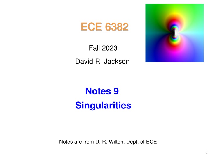
ECE 6382 Fall 2023 David R. Jackson Notes 9 Singularities Notes are from D. R. Wilton, Dept. of ECE 1
Singularity A point zs is a singularity of the function f(z) if the function is not analytic at zs. (The function does not necessarily have to be infinite there.) Recall from Liouville s theorem that the only function that is analytic and bounded everywhere in the complex plane is a constant. Hence, all non-constant functions that are analytic everywhere in the complex plane must be unbounded at infinity and hence have a singularity at infinity. ( ) f z ( ) = = z Example: e z x tends to infinity as 2
Taylor Series The radius of convergence Rc is the distance to the closest singularity. If f(z) is analytic in the region R c z z R 0z 0 c sz then ( ) f z ( ) n = a z z z z R for 0 n 0 c = 0 n ( )( ) ! n ( ) f z z n f z 1 0 = = a dz ( ) n + 1 n 2 i z C 0 The series converges for |z-z0| < Rc. The series diverges for |z-z0| > Rc (proof omitted). 3
Laurent Series b a z z b If f(z) is analytic in the region a 0 0z sz then sz ( ) f z ( ) n = a z z a z z b for 0 n 0 = n ( ) f z z 1 = a dz ( ) + n 1 n 2 i z C 0 The series converges inside the annulus. The series diverges outside the annulus (proof omitted). 4
Taylor Series Example Example: 1 y ( ) f z = 1 z 0z 1 ( ) f z x = = + + + + 2 3 1 z z z 1 z sz = 1 = n z The point z = 1 is a singularity (a first-order pole). = 0 n From the property of Taylor series we have: 1 = n , 1 z z 1 z = 0 n n diverges , 1 z z = 0 n 5
Taylor Series Example Example: y ( ) f z = z 1 x ( ) f z ( ) n = 1 a z Expand about z0 = 1: n = 0 n c R = 1 = = 1/2 1 a z 0 = 1 z 1 1 1! 2 1 2 1 2 1 8 1/2 = = a z ( ) ( ) 2 = + + 1 1 1 z z z 1 = 1 z 1 2! 2 1 1 2 1 8 3/2 = = a z z 1 1 2 The series converges for = 1 z etc. z 1 1 The series diverges for 6
Laurent Series Example Example: z y ( ) f z = 1 z ( ) f z ( ) 1 1 n = a z Expand about z0 = 1: x n = n Using the previous example, we have: = (The coefficients are shifted by 1 from the previous example.) 1 1 2 a 1 = a 1 1 2 1 8 z ( ) 0 = + + 1 z 1 1 z z 1 8 = a 1 The series converges for 0 1 1 z etc. z 1 1 The series diverges for 7
Isolated Singularity Isolated singularity: The function is singular at zs but is analytic for 0 z z s (for some ) 0 sz sin 1 z 1 z Examples: = 1/ z at , , , 0 e z sin z z A Laurent series expansion about zs is always possible! This is a special case of a Laurent series with . 0, a a b 8
Non-Isolated Singularity Non-Isolated Singularity: By definition, this is a singularity that is not isolated. y Example: 1 ( ) f z = 1 z sin x X X X X X X X X X ( X ( X X ) 1/ ) 1/ 1/ 2 1/ 2 Simple poles at: ( ) sz = 0 non-isolated singularity 1 (Distance between successive poles decreases with m !) = z m Note: The function is not analytic in any region 0 < |z| < . Note: A Laurent series expansion about z = 0 with a = 0 is not possible! 9
Non-Isolated Singularity (cont.) Branch Point: This is a type of non-isolated singularity. y Example: ( ) f z = 1/2 z x sz = 0 Not analytic at the branch point. Note: The function is not analytic in any region 0 < |z| < . Note: A Laurent series expansion in any neighborhood of z = 0 is not possible! 10
Examples of Singularities Examples: (These will be discussed in more detail later.) If expanded about the singularity, we can have: T = Taylor L = Laurent N = Neither ( ) z sin z removable singularity at z = 0 (isolated singularity) T 1 pole of order p at z = zs( if p= 1, pole is a simple pole) (isolated singularity) L ( ) p z z s 1/ z e essential singularity at z = 0 (pole of infinite order) L (isolated singularity) 1 non-isolated singularity z = 0 (fora = 0) N 1 z sin 1/2 z N non-isolated singularity z = 0 (branch point) 11
Classification of Isolated Singularities Isolated singularities Essential singularities (poles of infinite order) Removable singularities Poles of finite order 1 z 1 z 1 z 1 ( ) z z ( ) z 1 cos sin 1/ z sin , e , , , , ( ) 2 m 1 z 2 z + 2 1 ( 3 z z ( ) 2 + 2) z These are each discussed in more detail next. 12
Isolated Singularity: Removable Singularity Removable singularity: The limit z z0 exists and f(z) is made analytic by defining ( ) f z ( ) f z lim z 0 z 0 Example: ( ) z sin z sz L'Hospital's Rule ( ) z z ( ) 1 sin cos z = = lim z lim z 1 0 0 1 3 1 5 + 3 5 z z z ( ) z z sin 1 3 1 5 = = + 2 4 1 z z z Laurent series Taylor series 13
Isolated Singularity: Pole of Finite Order Pole of finite order (order P): ( ) f z ( ) n = a z z n s = n P sz The Laurent series expanded about the singularityterminates with a finite number of negative exponent terms. Examples: 1, ( z ( ) f z = = 1) P simple pole at z = 0 3 2 1 ( ) f z ( ) = + + + + + = 1 3 , ( 3) z P ( ) ( ) ( ) 3 2 3 z 3 3 z z pole of order 3 at z = 3 14
Isolated Singularity: Essential Singularity Essential Singularity (pole of infinite order): ( ) f z ( ) n = sz a z z n s = n The Laurent series expanded about the singularityhas an infinite number of negative exponent terms. Examples: n 1 z 1 n 1 z 1 z 1 z 1 ( ) f z ( ) + 1 n = = = + + sin 1 3 5 ! 6 120 z = 1 n odd n 1 1 ! n 1 z 1 z 1 z ( ) f z = = = + + + + 1/z 1 e 2 3 2 6 z = 0 n 15
Graphical Classification of an Isolated Singularity at zs Laurent series: ( ) f z ( ) ( ) ( ) ( ) ( ) 1 2 n p = = + + + + + + a z z a z z a z z a a z z a z z 1 0 1 2 n s p s s s s = n Analytic or removable Simple pole Isolated singularities Pole of orderp Essential singularity 16
Picards Theorem The behavior near an essential singularity is pretty wild! Picard s theorem: In any neighborhood of an essential singularity, the function will assume every complex number (with possibly a single exception) an infinite number of times. sz For example: ( ) f z 1/z e = No matter how small is, this function will assume all possible complex values (except possibly one). (Please see the next slide.) Charles mile Picard 17
Picards Theorem (cont.) n ( ) f z 1 1 ! n 1/z e = ( ) f z Example: = z = 0 n Set sz = 0 1/ z = = i e w R e a given arbitrary complex number) ( 0 0 0 Take the ln of both sides, equate real and imaginary parts. i er 1 r ( ) ( ) + cos s n i i 2 i n i = = = = = = 1/ z z re e e = e w R e 0 0 0 + ( ) cos ln , sin 2 r R r n 0 0 Any value of n gives a valid solution. ( ) 2 + = = + + 2 2 2 2 cos sin 1 ln 2 r R n 0 0 Hence ( ) + 2 n 1 n n = = 1 0 0, tan / 2 r ln R ( ) 2 + + 2 ln 2 R n 0 0 0 The exception here is w0 = 0 (R0 = 0). 18
Picards Theorem (cont.) y Example (cont.) ( ) f z 1/z e = sz = 0 x Note: A similar plot exists for negative n. n n = = 0, /2 r This sketch shows that as n increases, the points where the function exp(1/z) equals the given value w0 converge to the (essential) singularity at the origin. You can always find a solution for z now matter how small (the neighborhood ) is! 19
Picards Theorem (cont.) Example (cont.) ( ) f z 1/z e = re = i z cos sin 1/ z i = e e e r r Plot of the function exp(1/z), centered on the essential singularity at z = 0. The color represents the phase, the brightness represents the magnitude. This plot shows how approaching the essential singularity from different directions yields different behaviors (as opposed to a pole, which, approached from any direction, would be uniformly white). https://en.wikipedia.org/wiki/Essential_singularity 20
Picards Theorem (cont.) Compare with the behavior near a simple pole: 1 z 1 z 1 r ( ) f z = = i e 21
Singularity at Infinity We classify the types of singularities at infinity by letting w = 1/z and analyzing the resulting function at w = 0. Example: ( ) f z = 3 z 1 ( ) f z ( ) g w = = pole of order 3 at w = 0 3 w The function f(z) has a pole of order 3 at infinity. Note: When we say finite plane we mean everywhere except at infinity. The function f(z) in the example above is analytic in the finite plane. 22
Other Definitions Entire: The function is analytic everywhere in the finite plane. Examples: ( ) f z = + + 2 z , sin , 2 3 1 e z z z Meromorphic: The function is analytic everywhere in the finite plane except for isolated poles of finite order. sin 1 1 z z ( ) f z Examples: = = , ( ) g z ( )( ) 3 sin z + 1 z Meromorphic functions can always be expressed as the ratio of two entire functions, with the zeros of the denominator function as the poles (proof omitted). 23


")


")
")
")
")