Review of Definite Integrals using the Residue Theorem
Singular integrals involving logarithmic and non-integrable singularities are discussed, emphasizing integrability in the principal value sense. Cauchy Principal Value integrals and examples of their evaluations for singularities like 1/x are explored, highlighting the necessity of passing through the singularities for infinity cancellation. The importance of smooth functions in obtaining PV integrals is also noted.

Download Presentation

Please find below an Image/Link to download the presentation.
The content on the website is provided AS IS for your information and personal use only. It may not be sold, licensed, or shared on other websites without obtaining consent from the author.If you encounter any issues during the download, it is possible that the publisher has removed the file from their server.
You are allowed to download the files provided on this website for personal or commercial use, subject to the condition that they are used lawfully. All files are the property of their respective owners.
The content on the website is provided AS IS for your information and personal use only. It may not be sold, licensed, or shared on other websites without obtaining consent from the author.
E N D
Presentation Transcript
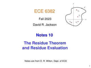
ECE 6382 Fall 2023 David R. Jackson Notes 11 Evaluation of Definite Integrals via the Residue Theorem Notes are from D. R. Wilton, Dept. of ECE 1
Review of SingularIntegrals Ln x 1 x ( ) z ( ) r = + i Ln ln Logarithmic singularities are examples of integrablesingularities: ( ) 1 1 1 ( ) x dx ( ) x dx ( ) x ( ) x = = = = Ln Ln Ln x 1 lim Ln x 0 x x since lim lim = 0 x 0 0 0 Note: There might be numerical trouble if one integrates this function numerically! 2
Review of SingularIntegrals (cont.) Singularities like 1/x are non-integrable. 1 x x 1 1 x 1 x ( ) 1 1 1 ( ) x = = = Ln dx dx lim lim = 0 x 0 0 3
Review of Cauchy Principal Value Integrals Consider the following integral: 1/ x dx x dx x dx x 2 0 2 0 2 = = + = + Ln Ln I x x 1 = = 1 0 x x x 1 1 0 2 A finite result is obtained if the integral interpreted as Excluded region ( ) dx x dx x dx x 2 2 = 2 = = + = + lim lim Ln Ln I x x =+ 1 x x 1 ( 1 0 0 ) = + Ln = lim Ln Ln1 Ln2 Ln2 0 The infinite contributions from the two symmetrical shaded parts shown exactly cancel in this limit. Integrals evaluated in this way are said to be (Cauchy) principal value (PV) integrals: or dx x dx x 2 2 = = PV I Notation: 1 1 4
Cauchy Principal Value Integrals (cont.) 1/x singularities are examples of singularities integrable only in the principal value (PV) sense. Principal value integrals must not start or end at the singularity, but must pass through them to permit cancellation of infinities 0 1/ x a x b Excluded region 5
Cauchy Principal Value Integrals (cont.) 2 1/ x Singularities like 1/x2 are non- integrable (even in the PV sense). x a b 1 x 1 x 1 a 1 1 1 b b + = + + dx dx 2 2 a 1 x , 0 x sgn( ) x x 2 = but note that has a PV integral 1 x 2 , 0 x 2 6
SingularIntegral Examples Summary of some results: Ln xis integrable at x = 0 1/x is integrable at x = 0 for 0 < < 1 1/x is non-integrable at x = 0 for f (x)sgn(x)/|x| has a PV integral at x = 0 for if f(x) is smooth (proof omitted) (The above results translate to singularities at a point a via the transformation x x-a.) 7
Integrals Along the Real Axis ( ) f x dx = I y i = = : , C z Re R Assumptions: i dz iRe d C fis analytic in the UHP except for a finite number of poles. x R R fis , i.e. in the UHP. ( ) 1/ o z lim z ( ) = 0 z f z UHP: Upper Half Plane On the large semicircle we then have Note: If the function is analytic in the LHP except for poles, then we would close the contour in the LHP. = = i i lim R ( ) f z dz lim R ( ) 0 f Re iRe d 0 C R Hence ( ) f x dx = = = = residues of in the UHP ( ) f z dz 2 ( ) f z I I i C C 8
Integrals Along the Real Axis (cont.) y Example: = = 3 2 z z i i 2 x dx = I ( )( ) 2 + + 2 2 9 4 x x 0 x = (Note the double pole at !) 2 z i 2 2 1 2 1 2 z dx z ( ) 3 + Res i ( ) 2 = = = 2 Res I dx i f f i ( )( ) ( )( ) 2 2 + + + + 2 2 2 2 9 4 9 4 z z z z 0 1 m 1 d dz = m Res ( ) f z ( ) ( ) f z z z ( ) 0 0 1 m 1 ! m 4 = z ( ) f z O z z = 0 ( ) ) ( ) 2 2 2 3 2 z i z z i z d dz = lim z + lim i ( ) ( ) ( 2 ( ) ( ) ( ) 2 2 3 2 i z i + + 2 + + 2 3 3 4 z i z i z 9 2 2 z z i z i ( ) ( )( ( ) ( ) ) ( + ) 2 2 + + + + + 2 2 2 9 2 2 9 2 2 2 2 z z i z z z z i z i z 3 + lim 50 i = i ( ) ( 2 ) 4 2 z i + + 2 9 2 z z i 3 50 13 200 i i 2 x dx = = i = = I 200 ( )( ) 2 200 + + 2 2 9 4 x x 0 9
Cauchy Principal Value Integrals ( ) f x dx = I C Assumptions: R R fis analytic in the UHP except for a finite number of poles. ( ) fis , i.e. in the UHP. ( ) 1/ o z lim z = 0 z f z A small semicircle of radius is introduced at a simple pole on the real axis. We let 0. Note: If the function is analytic in the LHP except for poles, then we would close the contour in the LHP. It is our choice to detour above or below the pole on the real axis. 10
Cauchy Principal Value Integrals Example = = i : , C z Re R C i dz iRe d dx = Evaluate: I ( )( ) + + 2 1 1 x x = z i z = 1 R R Consider the following integral: = z i ( ) i = = + = : 1 1 , C z z e i i e d I dz 1 R dz dz = = + + + lim R I ( )( ( )( ) ) C + + + + 2 2 1 1 1 1 z z z z , + 1 C R C C 0 R i 2 i e d i dz iRe d + = + + = + + lim R lim lim R I I ( )( ( )( ) ) ( ) + + + 2 2 2 2 i i 1 1 1 1 z z R e Re 0 + + i i 1 1 e e 0 C C 0 R 2 2 2 i i id ie d i ie d i = + + = + + = + + lim R lim R 0 I I I 2 2 2 2 2 R R 0 0 Hence, i We could have also used the formula from Notes 10 for going halfway around a simple pole on a small semicircle (the residue at -1 is 1/2). = + I I C 2 11
Cauchy Principal Value Integrals (cont.) = = i : , C z Re R dx C = I i dz iRe d ( )( ) + + 2 1 1 x x = z i z = 1 R R Next, evaluate the integral IC using the residue theorem: = z i + = = i : 1 , C z e i e d i dz ( ( ) )( i ( ) + ) ( 1 1 z i z = = ) Res ( + = = + 2 Res ( 1) 2 lim z lim z I i f z i f z i ( ( ) ) ) C + + + + 2 1 1 z i z z z z 1 i 1 1 2 1 1 2 1 1 2 i i = + = + = + = + 2 2 2 i i i i ( ) + 2 1 i 4 4 2 2 i i Hence: Recall: Thus: i = + = = + I I I CI i C 2 2 2 2 12
Fourier Integrals ( ) f x e dx y = iax I = = i : , C z Re R i dz iRe d a 0 Assume (close the path in the UHP) x Assumptions: R R f is analytic in the UHP except for a finite number of poles (can easily be extended to handle poles on the real axis via PV integrals), = lim ( ) 0, 0 arg z ( z ) f z z in UHP Choosing the contour shown, the contribution from the semicircular arc vanishes as R by Jordan s lemma. (See next slide.) Jean-Baptiste Joseph Fourier 13
Fourier Integrals (cont.) Jordan s lemma y = = i : , C z Re R i dz iRe d Assume = lim ( ) z 0, 0 arg ( z ) f z z in UHP x R ( ) f z e dz iaz Then R 0 C R Proof: /2 ( ) i i i = cos sin sin iaz iaR aR aR ( ) f z e dz ( ) 2 max ( ) f Re e e iRe d R f Re e d 0 0 C R /2 2 aR ( )max ( ) ( ) i i e = aR 2 max ( ) 2 ( ) 1 0 R f Re e d R f Re 2 a R 0 2 1 2 aR 2 sin sin aR 0 / 2: sin e e 2 14
Fourier Integrals (cont.) ( ) f x e dx = y iax I = = i : , C z Re R i dz iRe d ( ) f z e dz iaz 0 x C R R R We then have C = = = e e iaz iaz ( ) f z 2 ( ) f z I I dz i residues of in the UHP C Questions: What would change if a < 0 ? If we had a negative sign in the exponential? 15
Fourier Integrals (cont.) y Example: + cos x x ( ) = , , 0. I dx a 2 2 z = a ia 0 x i x = x i + cos sin e x Note: Use the symmetries of cos( x) and sin( x) and the Euler formula, we have: i x 1 2 e = (imaginary part vanishes by symmetry!) I dx + 2 2 x a ( + ) z i z z ia ) ( e i z i z 1 2 1 2 1 2 e e = = 2 Res = 2 lim z I dz i i ( ) + + 2 2 2 2 z a z a z ia ia ia z ia = a a 1 2 2 e e + a cos x x e = = 2 i = = I 2 a i a 2 2 2 a a 0 16
Rational Functions of sin and cos 2 ( ) = sin ,cos f d I Assumptions: 0 f is finite within the interval. f is a rational function (ratio of polynomials) of sin , cos . dz z = = = i i Let , z e dz ie d d i unit circle + 1 1 z z i z z = = sin , cos 2 2 2 + 1 1 z z i z z dz z ( ) = sin ,cos = f d i , I f 2 2 = 0 1 z + 1 1 1 z z z i z z = Residues of inside the unit circle 2 , f 2 2 + 1 1 1 z z z i z z will be a rational function of Note: , f z 2 2 17
Rational Functions of sin and cos (cont.) y Example: z = 1 d 2 = I + sin 5 4 0 x = z i 1 2 1 d dz z 2 = = I i + + 1 sin z z Multiply top and bottom by 4i. 5 4 5 4 0 = 2 i 1 z = 2 z i 4 2 4 2 i z dz ( ) = idz = )( ( + ) ) + ( + + + 2 5 2 2 iz z i z i 1 2 = = 1 1 z z = + ) ( i 2 z i 1 2 2 i 8 dz = = 2 lim i )( ) ( ) ( + + 2 3 z z i 1 2 2 z z i 1 2 1 2 z i = 1 z 8 d 2 Note: = = I The poles (roots of the denominator) are found by using the quadratic equation. + sin 3 5 4 0 18
Exponential Integrals There is no general rule for choosing the contour of integration; if the integral can be done by contour integration and the residue theorem, the contour is usually specific to the problem. y = 3 z i Example: 3 = 2 z i ax e + = 4 , 0 1 I dx a 2 = z i 1 x 1 e x R R Consider the contour integral over the path shown in the figure: = = + + + + az az e e + The integrand has simple poles at I dz dz C z z 1 1 e e z = = + = 0, 1, 2, 1 2 , e z i n n C 1 2 3 4 R The contribution from each contour segment in the limit must be separately evaluated (next slide). 19
Exponential Integrals (cont.) y = = 1: , , z x dz dx R = 3 z i az e + = lim R dz I 3 = 2 z i z 1 e 1 4 2 = z i 1 x R = + = : 2 , , z x i dz dx R 3 R az ax e + e + = = 2 2 ia ia lim R lim R dz e dx e I z x 1 1 e e R 3 = R iy + = : , z dz idy 2 2 ( ) 1 az aR iay e e e e + e + + R iy R e e e = dz i dy z R iy 1 1 e 0 2 ( ) aR iay e e + aR iay e e 2 2 2 2 1 a R aR e e = = 0, 1 dy dy dy dy a R R + 1 1 R iy e e iy R iy e e 1 e e e 0 0 0 0 20
Exponential Integrals (cont.) y = + = : , , z R iy dz idy 4 3 = 2 z i 0 az aR iay e e e e + e + = dz i dy z R iy 1 1 e 4 2 = z i 2 1 4 x 2 aR e R R 0, 0 dy a R 1 e 0 ( ) ( ) h z g z ( ) ) ) = = Alternatively, ( ) f z , 0 h z ( ) 0 + R iy R 1 1 e e e ( ( az g z h z e 0 = = = Res ( ) lim z lim z f z i ( ) d dz z i z + 0 1 e 0 Hence a i a i e e e a i = = = e i 1 ( ) ( ) = = 2 ia 1 2 Res e I i f z i az az az e + e e e ( ) ( ) ( ) ( ) = = z i = z i = z i Res lim z lim z lim z f z i z i + z i + z i 1 1 1 e e i i i ( ) z i az e ( az e z i = = = ia lim z lim z e ( ) ( ) ) 1 2 1 2 + + z i + i i 1 1 z i 1 2 21
Exponential Integrals (cont.) We thus have ( ) = 2 ia ia 1 2 e I ie Therefore ax ia ia 2 2 e e + ie e i e = = = = , 0 1 I dx a ( ) 2 x ia 1 1 sin e a ia ia ia e e Hence ax e + = = , 0 1 I dx a x 1 sin e a 22
Integration Around a Branch Cut A given contour of integration is chosen: usually problem specific, usually must not cross a branch cut. We take advantage of the fact that the integrand changes across the branch cut. Usually an evaluation of the contribution from the branch point is required. y Example: k x = , 0 1 I dx k + 1 x 0 z = 1 x Assume the branch 0 < 2 ( x = positive real) k ( ) k ( ) ( ) r i + ln ln ( ) k k r = = = = ln ln k x k x ( x e e e e = ) 0 x on the axis Note: We choose the branch cut on the positive real axis (the axis of integration). 23
Integration Around a Branch Cut (cont.) k x x = , 0 1 I d x k + 1 0 First, note the integral exists since the integral of the asymptotic forms of the integrand at both limits exists: k x = k which is integrable at 0, 1 x x k + 0 x 1 k x x = 1 k which is integrable at , 0 x x k + x 1 x 24
Integration Around a Branch Cut 1 x 1 r ( ) k x = = = 0 k i Note: x x re (principal branch) = , 0 1 I dx k k k + 1 x y 0 We ll evaluate the integral using the contour shown. 0 1 L 0r z = 1 x 0 2 C 0 L 2 2 R C For either circle, use: R ( ) i = = z re r r R or 0 ( ) k ( ) r i + ln k = = = = = ln ln ln k k z k r ik r ik k ik , 0 2 z e e e e e e r e = k k ik , 0 2 z r e 25
Integration Around a Branch Cut (cont.) y Now consider the various contributions to the contour integral: ( ) f z dz ( ) = 1 , 2 Res i f 0 + + + L C L C 1 2 0 R 1 L k z 0r ( ) f z z = 1 = where x + C 1 z 0 L 2 2 = k k ik , 0 2 z r e R C R i i = = = k k ik : , , C z r e dz ir e d z r e 0 0 0 0 0 i k ik r e ir e d + ( ) f z dz = = 1 k i ik 0 0 lim r lim r 0 ir e d 0 i 1 r e 0, 0 0 0 0 0 2 2 C 0 i i = = = k k ik : , , C z Re dz iRe d z R e R 2 2 k ik i R e iRe d + ( ) f z dz = = k ik lim R lim R 0 iR e d i 1 Re , 0 C 0 R 26
Integration Around a Branch Cut (cont.) k z ( ) f z = = k k ik , 0 2 z r e y + 1 z For the path L1: = = = i i k k ik 1: , , L z re dz e dr z r e 0 1 L 0r z = 1 R k k r re dr + r dr + x ( ) f z dz = = = ( ) i k lim R r e I C 0 i 1 1 r L 2 0 L r 2 0 0 1 0 0 R C R For the path L2: ( ) ( ) 2 2 i ik = = = = i i k k 2: , , L z re re dz e dr z r e r k k r dr r dr + 0 ( ) f z dz + (2 ) i k = = = 2 2 i k i k lim R r e e e I + i 1 1 re r 0 L R 0 0 2 0 27
Integration Around a Branch Cut (cont.) Hence ( ) ( ) = = 2 i k 1 2 Res 1 e I i f z k z ( ) = + 2 lim z ( ( i e ie 1 i z + 1 z 1 ) ) k = 2 1 i k = i 2 Note: Arg (-1) = here (0 < < 2 ). = ik 2 Therefore, we have ( ik ik 2 1 2 ie e i e e = = = , 0 1 I k ( ) ) 2 i k sin k i k ik ik e e Hence k x = = , 0 1 I dx k + 1 sin x k 0 28
Hilbert Transforms y 0 CI C Assumptions: R C ( ) ( ) f z = + is analytic in the UHP f z u iv (including the real axis) R R 0 in the UHP 0 , z 0x UHP: Upper Half Plane x R R Consider: ( ) i f x CPV 0 ( ) = ( ) z x ( ) x + i x f x e 2 R f f 0 ( ) 0 i e = + + i f x i lim R 2 dz dx d 0 z x x i e 0 0 + C R x 0 0 ( ) f x x ( ) ( ) + i f x = i f x 2 dx 0 0 x (From the residue theorem or the Cauchy integral theorem.) 0 ( ) f x x e = i Let z x 1 ( ) f x = 0 dx 0 i x 0 ( ) v x x ( ) u x x 1 i + = ( ) ( ) u x iv x dx dx 0 0 x x 0 0 29
Hilbert Transforms (cont.) ( ) v x x ( ) u x x 1 i ( ) f x = + = ( ) ( ) u x iv x dx dx 0 0 0 x x 0 0 Equate the real and imaginary parts: ( ) v x x 1 = ( ) u x dx 0 x 0 ( ) u x x 1 = ( ) v x dx 0 x 0 Next, relabel: , x x x x 0 30
Hilbert Transforms (cont.) Hence, we have ( ) v x x 1 = ( ) u x dx x ( ) u x x 1 = ( ) v x dx x David Hilbert are Hilbert Transforms of one another ( ), ( ) u x v x Assumptions: ( ) ( ) f z = + is analytic in the UHP f z u iv (including the real axis) in the UHP 0 , z 31
Hilbert Transforms (cont.) We can also repeat the derivation assuming that the function is analytic in the lower half plane. Im ( ) v x x 1 = ( ) u x dx x ( ) u x x 1 R R = ( ) v x dx Re 0x x C Assumptions: ( ) ( ) z = + is analytic in the LHP f z u iv (including the real axis) in the LHP 0 , f z 32
Hilbert Transforms in Circuit Theory (using j instead of i) + ( ) = ( ) + ( ) + H H j H R I in( ) V out( ) V Im Transfer function Poles are only allowed in the UHP. ( ) ( ) ( ) / H V V out in ( ) j t Assumpti on s : exp( ) time convention ( ) 1 Re ( ) is an alytic in the LHP H ( ) 2 f or in the LHP ( ) 0, H LHP: Lower Half Plane Note 1: A pole in the LHP would corresponds to a nonphysical growing response: j e = + j t = t j t e e i r r i Note 2: The system is assumed to be unable to respond to a signal at very high frequency. ( ) ( ) ( ) ( ) ( ) ( ) = = = Symmetry property: * ; H H H H H H R R I I (see Appendix) 33
Hilbert Transforms in Circuit Theory (cont.) We thus have: + ( ) = ( ) + ( ) + H H j H R I in( ) V out( ) V Transfer function ( ) ( ) ( ) / H V V out in ( ) H 1 ( ) = I H d R ( ) H 1 ( ) = R H d I The real and imaginary parts of the transfer function are Hilbert transforms of each other. 34
Hilbert Transforms in Circuit Theory (cont.) We can also derive an alternative form: ( ) ( ) ( ) 0 H H H 1 1 1 ( ) = = I I I H d d d R First one: Use 0 H ( ) ( ) 0 H 1 1 = I I d d First one: Use 0 ( ) ( ) ( + ) ( ) = H H H H 1 1 I I = I I d d 0 0 ) ( ( ( )( ) ( ) ( + ) + + H 1 I = d )( ) 0 ( ) 2 H 1 = I d This integral starts at zero. ( ) 2 2 0 Similarly, we have ( ) ( )( 2 ) 2 H H 1 1 ( ) = = R R H d d ( ) I 2 0 35
Dispersion Relation: Circuit Theory (cont.) Summarizing, we have: ( ) ( ) H H 1 2 ( ) = = I I H d d ( H ) R 2 2 0 ( ) ( ) H 1 2 ( ) = = R R H d d ( ) I 2 2 0 Assumption s: is analytic in the LHP fo ( ) ( ) H H r in t he LHP 0, 36
Kramers-Kronig Relations Hendrik Anthony Hans Kramers Ralph de Laer Kronig The Kramers-Kronig relations are a fundamental set of equations that relate the real and imaginary parts of the complex permittivity. 37
Kramers-Kronig Relations Assumption: The relative permittivity is analytic in the LHP and in LHP ( ) ( ) 1, r r Similar to the transfer-function analysis, one obtains the Kramers-Kronig dispersion relations: ( ) ) 1 Im ( 2 ( ) ( ) 1 = r Re d r 2 2 0 ( ) ) 1 Re ( 2 ( ) ( ) 1 = r Im d r 2 2 0 Material parameters: relative permittivity electric susceptibility = P E (polarization per unit volume) r 0 e e e ( ) 0 as in LHP ( ) 1 ( ) e r 38
Kramers-Kronig Relations (cont.) ( ) r = using instead of ( ) ( ) ( ) j j i Denote r r The final form of the Kramers-Kronig relations is then: ( ) 2 ( ) r = + r 1 d 2 2 0 ( ) ( ) 2 1 2 ( ) r = d r 2 0 Note: This shows that if there is no loss ( r = 0), then the relative permittivity must be 1. Hence, practical materials with r > 1 will always have some loss. 39
Laplace Transform The Laplace transform is defined as: ( ) ( ) st F s f t e dt 0 ( ) Assume Im s ( ) t 0, 0 f t Ae t Analytic Then F(s) is analytic in the region ( ) ( ) Re s Re s 0 0 ( ) ( ) ( ) t f t e dt ( ) F s = Re > s st Note: valid for 0 0 Note: In the Laplace transform we do not care how f is defined for t< 0. 40
Laplace Transform (cont.) Define a function g(t) (using any > 0): t ( ), 0 0 e f t t t The Fourier transform of g(t) exists. (The function g(t) stays finite along the entire real axis and tends to zero as t .) ( ) g t 0, We then have, from the inverse Fourier transform, 1 ( ) ( ) ( ) i t = Im s ( ) ( ) g t g e d i t g g t e d 2 C Then, from the relation between f and g: 1 ( ) ( ) t i t = , 0 f t g e e d t 2 ( ) Re s + s i Let + i 1 ( ) ( ) ( ) = i s st , 0 f t g e ds t 2 i i 41
Laplace Transform (cont.) + i 1 ( ) ( ) ( ) = i s st , 0 f t g e ds t 2 i i We have for the integrand term: ( ) Im s ( ) ( ) ( ) ( ) ( ) i i s t i s = g g t e dt C ( ) ( ) ( ) i i s t = g t e dt 0 ( ) Re s ( ) ( ) s t = g t e dt 0 ( ) = st f t e dt 0 F s ( ) = 42
Laplace Transform (cont.) Hence, we have: + i 1 ( ) ( ) t ( ) = st , 0 f t f F s e ds t Inverse Laplace transform B 2 i i ( ) Im s Bromwich integral C The Bromwich contour C is chosen to the right of all singularities of the function F(s). ( ) Re s ( ) t 0, 0 f t Ae t 0 43
Laplace Transform (cont.) Consider the case: + i 1 ( ) t ( ) t st f F s e ds 0 B 2 i i Close the contour to the right. C The integrand is analytic inside . R : C Only the vertical path contributes as C R ( ) Im s st Right: Top and bottom: 0 e ( ) 0 ( ) F s assumption C R 1 ( ) t ( ) = st f F s e ds C B 2 i ( ) C Re s R ( ) t = 0 Bf (by Cauchy s theorem) 44
Laplace Transform (cont.) Summary ( ) Im s ( ), f t t + i 0 t 1 ( ) t ( ) = = st f F s e ds C B 2 i 0, 0 i ( ) Re s Note: This inverse Laplace transform (Bromwich) integral gives us zero for t < 0, no matter how the original function f(t) was defined for t < 0. 45
Laplace Transform (cont.) Evaluation of the Bromwich integral for the case of poles only: + i 1 ( ) ( ) t ( ) t 0 = = st f t f F s e ds B 2 i i Close the contour to the left. ( ) : C Only the vertical path contributes as C Im s L st Left: Top and bottom: 0 e ( ) C 0 ( ) F s L assumption C 1 ( ) ( ) = st f t F s e ds ( ) Re s 2 i C L ( ) f t = residues at poles to the left of C Poles only (This assumes that there are only pole singularities.) 46
Laplace Transform (cont.) ( ) = at Example f t e = Note: a a 0 1 ( ) ( ) ( ) s a t s a t = = = at st F s e e dt e dt e s a 0 0 0 1 ( ) ( ) ( ) s Im s = , Re F s a s a C For t > 0: L + i 1 1 ( ) ( ) t = = st , f t f e ds a B 2 i s a ( ) a Re s i 1 1 ( ) t = st 2 Res f i e B 2 i s a s a = ( ) t = at , 0 Bf e t 47
Appendix ( ) ( ) Proof of symmetry property: = * H H + ( ) = ( ) + ( ) + H H iH R I in( ) V out( ) V Transfer function ( ) ( ) ( ) / H V V out in Impulse response: 1 ( ) ( ) ( ) ( ) = i t = = i t h t H e d H h t e dt real 2 = Use so 1 1 1 1 ( ) ( ) ( ) ( ) ( ) ( ) i t i t i t i t = = = = = * * * * * h t h t H e d H e d H e d H e d 2 2 2 2 Relabel Hence: 1 1 ( ) ( ) ( ) ( ) ( ) ( ) i t i t = = * 1 1 * = * H e d H e d F H F H H H 2 2 48


")

")
")


")


")

")
")
")

")

")
")
")

")

")
")
")

")
")
")

")
")
")


")

")
")
")
")
")
")
")