Rooted Trees in Discrete Structures
In this study material, you will delve into the concept of trees in discrete structures, focusing on rooted trees with recursive definitions and terminology. Discover the important properties of trees and explore how they are used as models, such as in the Domain Name System and computer file systems. Learn about binary and m-ary trees, including their characteristics and full tree scenarios. Dive into the properties of trees and explore the theorems related to the number of nodes and edges in a tree.

Uploaded on Feb 25, 2025 | 0 Views
Download Presentation

Please find below an Image/Link to download the presentation.
The content on the website is provided AS IS for your information and personal use only. It may not be sold, licensed, or shared on other websites without obtaining consent from the author.If you encounter any issues during the download, it is possible that the publisher has removed the file from their server.
You are allowed to download the files provided on this website for personal or commercial use, subject to the condition that they are used lawfully. All files are the property of their respective owners.
The content on the website is provided AS IS for your information and personal use only. It may not be sold, licensed, or shared on other websites without obtaining consent from the author.
E N D
Presentation Transcript
22C:19 Discrete Structures Trees Fall 2014 Sukumar Ghosh
Rooted tree terminology (If u = v then it is not a proper descendant) If v is a descendant of u, then u is an ancestor of v
Rooted tree terminology A subtree
Important properties of trees Theorem. A tree with n nodes has (n-1) edges Proof. Try a proof by induction
Important properties of trees Theorem. A tree with n nodes has (n-1) edges Proof. Try a proof by induction
Trees as models Domain Name System
Trees as models directory subdirectory subdirectory subdirectory file file file file file file file file file Computer File System This tree is a ternary (3-ary) tree, since each non-leaf node has three children
Binary and m-ary tree Binary tree. Each non-leaf node has up to 2 children. If every non-leaf node has exactly two nodes, then it becomes a full binary tree. m-ary tree. Each non-leaf node has up to m children. If every non-leaf node has exactly m nodes, then it becomes a full m-ary tree
Properties of trees Theorem. A full m-ary tree with k internal vertices contains n = (m.k + 1) vertices. Proof. Try to prove it by induction. [Note. Every node except the leaves is an internal vertex]
Properties of trees Theorem. Every tree is a bipartite graph. Theorem. Every tree is a planar graph.
Balanced trees The level of a vertex v in a rooted tree is the length of the unique path from the root to this vertex. The level of the root is zero. The height of a rooted tree is the maximum of the levels of vertices. The height of a rooted tree is the length of the longest path from the root to any vertex. A rooted m-ary tree of height h is balanced if all leaves are at levels h or h 1.
Balanced trees Theorem. There are at most mhleaves in an m-ary tree of height h. Proof. Prove it by induction. Corollary. If an m-ary tree of height h has l leaves, then If the m-ary tree is full and balanced, then
Binary search tree Ordered binary tree. For any non-leaf node The left subtree contains the lower keys. The right subtree contains the higher keys. How can you search an item? How many steps does each search take? A binary search tree of size 9 and depth 3, with root 8 and leaves 1, 4, 7 and 13
Insertion in a binary search tree procedure insertion (T : binary search tree, x: item) v := root of T {a vertex not present in T has the value null } while v null and label(v) x if x < label(v) then if left child of v null then v := left child of v else add new vertex as a left child of v and set v := null else if right child of v null then v := right child of v else add new vertex as a right child of v and set v := null if root of T = null then add a vertex v to the tree and label it with x else if v = null or label(v) x then label new vertex with x and let v be the new vertex return v {v = location of x}
Decision tree Decision trees generate solutions via a sequence of decisions. Example 1. There are seven coins, all of which are of equal weight, and one counterfeit coin that is lighter than the rest. Given a weighing scale, in how many times do you need to weigh (each weighing determines the relative weights of the objects on the the two pans) to identify the counterfeit coin? {We will solve it in the class}.
Comparison based sorting algorithms A decision tree for sorting three elements
Comparison based sorting algorithms Theorem. Given n items (no two of which are equal), a sorting algorithm based on binary comparisons requires at least comparisons Proof. See page 761-762 of your textbook. We will discuss it in the class The complexity of such an algorithm is Why?
Spanning tree Consider a connected graph G. A spanning tree is a tree that contains every vertex of G Many other spanning trees of this graph exist
Computing a spanning tree Given a connected graph G, remove the edges (in some order) without disrupting the connectivity, i.e. not causing a partition of the graph. When no further edges can be removed, a spanning tree is generated. Graph G
Computing a spanning tree Spanning tree of G
Depth First Search procedureDFS (G: connected graph with vertices v1 vn) T := tree consisting only of the vertex v1 visit(v1) {Recursive procedure} procedurevisit (v: vertex of G) for each vertex w adjacent to v and not yet in T add vertex w and edge {v, w} to T visit (w) The visited nodes and the edges connecting them form a spanning tree. DFS can also be used as a search or traversal algorithm
Breadth First Search Given graph G A different way of generating a spanning tree Spanning tree
Breadth First Search ALGORITHM. Breadth-First Search. procedureBFS (G: connected graph with vertices v1, v2, vn) T := tree consisting only of vertex v1 L := empty list put v1 in the list L of unprocessed vertices while L is not empty remove the first vertex v from L for each neighbor w of v if w is not in L and not in T then add w to the end of the list L add w and edge {v, w} to T
Minimum spanning tree A minimum spanning tree (MST) of a connected weighted graph is a spanning tree for which the sum of the edge weights is the minimum. How can you compute the MST of a graph G?
Huffman coding Consider the problem of coding the letters of the English alphabet using bit-strings. One easy solution is to use 5 bits for each letter (25 > 26). Another such example is The ASCII code. These are static codes, and do not make use of the frequency of usage of the letters to reduce the size of the bit string. One method of reducing the size of the bit pattern is to use prefix codes.
Prefix codes In typical English texts, e is most frequent, followed by, l, n, s, t The prefix tree assigns to each letter of the alphabet a code whose length depends on the frequency: 0 1 0 e 1 a 0 1 l 0 1 e = 0, a = 10, l= 110, n = 1110 etc n 1 0 Such techniques are popular for data compression purposes. The resulting code is a variable-length code. s t
Huffman codes Another data compression technique first developed By David Huffman when he was a graduate student at MIT in 1951. (see pp. 763-764 of the textbook) Huffman coding is a fundamental algorithm in data compression, the subject devoted to reducing the number of bits required to represent information.
Huffman codes Example. Use Huffman coding to encode the following symbols with the frequencies listed: A: 0.08, B: 0.10, C: 0.12, D: 0.15, E: 0.20, F: 0.35. What is the average number of bits used to encode a character?
Huffman coding example So, what is the average number of bits needed to encode each letter?