Regression Discontinuity Designs in Applied Economic Research

Regression Discontinuity Designs in
Applied Economic Research
Dr. Kamiljon T. Akramov
IFPRI, Washington, DC, USA
Regional Training Course on Applied Econometric Analysis
June 12-23, 2017, WIUT, Tashkent, Uzbekistan
Outline
•
Introduction and origins of RDD
•
Meaning and validity of RDD
•
Several examples from the literature
•
Estimation (where most decisions are made)
•
Discussion of a paper
•
Stata code and data will be provided
•
Conclusions
… when you start exercising those rules, all sorts
of processes start to happen and you start to find
out all sorts of stuff about people…. It’s just a way
of thinking about a problem, which let’s the shape
of the problem begin to emerge. The more rules,
the more arbitrary they are, the better.
Douglas Adams,
Mostly Harmless
Introduction
•
RDD allows to estimate causal treatment effects in non-experimental settings
•
It exploits precise knowledge of the rules determining treatment
•
Identification is based on the idea that some rules are arbitrary and provide
good quasi experiments
•
Randomized variation in RDD is a consequence of agents’ inability to precisely
control the assignment variable near the known cutoff point
•
RDD provides very good internal validity but external validity is limited
•
Recent flurry of applied economics research using RDD
•
Seemingly mild assumptions (Hahn, Todd, and van der Klaauw 2001)
•
More credible than other non-experimental identification strategies (Lee 2008)
Introduction (cont.)
•
RDD will be invalid if agents can precisely manipulate the “assignment
variable rule)”
•
If agents – even while having some influence – cannot precisely
manipulate the assignment variable RDD will be valid
•
RDD can be easily estimated and tested like RCTs
Origins of RDD: Thistlethwaite and Campbell (1960)
•
This was a first application of RD design
•
Impact of merit awards on future academic outcomes (career aspirations, enrollment in
postgraduate programs, etc.)
•
The study exploited the fact that awards were allocated on the basis of test scores
•
If a person had a score greater than c, the cutoff point, then she or he received the
award, while those with scores below c denied the award
•
Simple approach to the analysis: compare those who received the award to those who
didn't
•
Why is this the wrong approach?
•
Factors that influence the test score are also related to future academic outcomes (HH income,
parents' education, motivation, etc.)
•
Thistlethwaite and Campbell realized they could compare individuals just above and
below the cutoff point
Origins of RDD: Thistlethwaite and Campbell
(1960): Validity
•
Simple idea: assignment mechanism is known
•
We know that the probability of treatment jumps to 1 if test score ≥ c
•
Assumption is that individuals cannot manipulate with precision their assignment
variable (think about standardized tests: SAT, GRE, GMAT)
•
Individuals near cutoff point seem comparable and there appears to be no reason,
other than the merit award, for future academic outcomes to be discontinuous
function of test scores
•
This suggests attributing the discontinuous jump in outcome variables at c to the causal
effect of merit award
•
If treated and untreated individuals are similar near the cutoff point then data can be
analyzed as if it were a (conditionally) randomized experiment
Origins of RDD: Thistlethwaite and Campbell
(1960): Validity (cont.)
•
If this is true, then background characteristics of individuals should be
similar near the cutoff point (can be checked empirically)
•
The estimated treatment effect applies to those near the cutoff point,
which limits the external validity
•
Validity hinges on assignment mechanism being known and free of
manipulation with precision or cutoff point in some way related to
outcome of interest
•
Manipulation and validity
•
Some manipulation is fine (you can always study harder, for example)
•
Precision and lack of relation of the cutoff point to outcome is the key to
identify the causal effect
Identification in RDD
•
Two important features of identification in RDD
•
First
•
All other factors determining the outcome variable should be evolving
smoothly with respect to the assignment variable (rule)
•
If other factors (variables) also jump at the cutoff point, then the estimates of
treatment effect will be biased
•
Second
•
Since RD estimate requires data away from c, the estimate will be dependent
on a chosen functional form
Sharp and Fuzzy Discontinuity RDDs
•
Sharp discontinuity
•
The discontinuity precisely determines treatment, i.e., probability of treatment
jumps from 0 to 1 when X crosses the threshold
•
Equivalent to random assignment in a neighborhood
•
Example: Social security payment depends directly and immediately on a
person’s age
•
Fuzzy discontinuity
•
Discontinuity is highly correlated with treatment
•
Probability of treatment jumps by less than one when X crosses the threshold
•
Example: Rules determine eligibility but there is a margin of administrative
error
•
Use the assignment rule as an IV for program participation
Sharp RD
Discontinuity example
•
National Merit Scholarship awards in USA
•
National Merit Scholarship Corporation (NMSC) uses PSAT/NMSQT
scores as the initial screen of over 1.5 million program entrants
•
NMSC determines a national Selection Index qualifying score
(critical reading + math + writing skills scores) for "Commended"
recognition
•
Qualifying score is calculated each year to yield students at about
the 96th percentile (top 50,000 highest scorers)
•
Basically the top test-takers get a scholarship
•
A small difference in test score means a discontinuous jump in
scholarship amount
Identification for sharp discontinuity
Y
i
=
β
0
+
β
1
D
i
+ β
2
X
i
+ ε
i
D
i
=
Assignment rule under sharp discontinuity:
D
i
= 1
D
i
= 0
Identification for sharp discontinuity (cont.)
Counterfactuals
Counterfactuals (cont.)
Extrapolation (dashed lines)
When to use sharp RD design
•
The beneficiaries/non-beneficiaries can be ordered along a quantifiable
dimension
•
This dimension can be used to compute a well-defined index or parameter
•
The index/parameter has a cut-off point for eligibility
•
The index value is what drives the assignment of a potential beneficiary to
the treatment or to non-treatment groups
Indexes are common in targeting of welfare
programs
Anti-poverty
programs
Pension
programs
Scholarships
CDD programs
targeted to households below a given
poverty index
targeted to population above a certain
age
targeted to students with high scores
on standardized test
awarded to NGOs that achieve highest
scores
Example: Effect of cash transfers on
consumption
•
Objective: Target transfers to poorest households
•
Method
•
Construct poverty index from 1 to 100 with pre-intervention characteristics
•
Households with a score ≤ 50 are poor
•
Households with a score >50 are non-poor
•
Evaluation
•
Measure outcomes (i.e., consumption, school attendance rates, nutrition
outcomes)
before and after transfer, comparing households just above and
below the cut-off point
Regression Discontinuity Design-Baseline
Not Poor
Poor
Regression Discontinuity Design-Post Intervention
Treatment
Effect
Identification for fuzzy discontinuity
Y
i
= β
0
+
β
1
D
i
+
δ
X
i
+ ε
i
D
i
=
1
If household receives transfer
0
If household
does not
receive transfer
But
Treatment depends on whether
X
i
≥ or< c and other factors.
Since probability of treatment jumps by less than one at the threshold,
relationship between Y and D cannot be interpreted as average treatment effect.
As in IV setting, the treatment effect can be recovered by dividing the change in
the relationship between Y and D at c by fraction induced by treatment at the
threshold.
Identification for fuzzy discontinuity (cont.)
Y
i
= β
0
+
β
1
D
i
+ f(X
i
) + ε
i
First stage:
D
i
= γ
0
+ γ
1
I
(X
i
≥ c)
+ η
i
y
i
= β
0
+
β
1
D
i
+ f(X
i
) + ε
i
Second stage:
IV estimation
Dummy variable
Continuous
function
Examples from literature
Do benefits of additional medical expenditures exceed their
costs? (Almond et al. QJE, 2010)
•
RDD allows to compare health outcomes and medical treatment provision for
newborns on either side of the very low birth weight threshold at 1,500 grams
•
Study finds that newborns with birth weights just below 1,500 grams
have
lower
one-year mortality rates than do newborns with birth weights just
above this cutoff, even though mortality risk tends to decrease with birth weight
•
One-year mortality falls by approximately one percentage point as birth weight
crosses 1,500 grams from above
•
Infants with birth weight < 1,500 grams receive more medical treatment and their
hospital costs higher by $4,000 relative to mean hospital costs of $40,000 for
infants with birth weight just above 1,500 grams
•
Assuming observed medical spending fully captures the impact of the “very low
birth weight” designation on mortality, the study estimates suggest that the cost
of saving a statistical life of a newborn with birth weight near 1,500 grams is on
the order of $550,000 in 2006 dollars
Economic impact of unionization
(DiNardo &
Lee, QJE 2004)
•
Estimation of economic impacts of unionization is difficult due to selection bias
•
Unions could organize at highly profitable enterprises that are more likely to grow
and pay higher wages
•
Union elections
•
If employers want to unionize, board holds election
•
50% or less means the employer doesn’t have to recognize the union, and
•
50% + 1 means the employer is required to “bargain in good faith” with the
union
•
Multiple establishment-level datasets that represent establishments
that faced organizing drives in the United States during 1984-1999
Economic impact of unionization
DiNardo &
Lee, QJE 2004 (cont.)
•
The paper applies RD design to estimate the impact of unionization
on business survival, employment, output, productivity, and wages
•
Paper essentially compares outcomes for employers where unions
barely won the election with those where the unions barely lost
•
The analysis finds small impacts on all outcomes
•
The results suggest that-at least in the study period-the legal mandate
that requires the employer to bargain with a certified union has had
little economic impact
Effects of class size on test scores (Angrist &
Levy, QJE 1999)
•
Fuzzy RD design is used to estimate the effects of class size on student’s test scores
•
School class size- Maimonides’ rule
•
No more than 40 kids in a class in Israel
•
40 kids in school means 40 kids per class
•
41 kids means two classes with 20 and 21 kids
•
Multiple discontinuities: causal variable of interest, class size, takes on many values
•
Nonlinear relationship between the local number of students and the class size predicted by
Maimonides' rule to estimate the impact of class size on student performance, and evaluate the
effect of being just below the number of students for whom an additional teacher would be
brought up, and of being just above this number
•
First stage exploits jumps in average class size
•
Finding: smaller class size increases test scores
•
The results have shown highly irregular patterns in class size that are precisely mirrored in
student achievement: a reduction in predicted class size of ten students is associated with a
0.25
standard deviation
increase in fifth-graders' test scores
RD examples from literature (cont.)
•
Anderson and Magruder (2012) and Lucas (2012)
•
Yelp.com ratings have an underlying continuous score
•
Distribution determines cutoff points for 1 to 5 stars
•
Effect of an extra star on future reservations and revenue
•
Anderson et al. (2012)
•
Young adults lose their health insurance as they age (older than 18 and in
college but different after ACA)
•
Age changes the probability of having health insurance (fuzzy design)
Paper by
Raffaello Bronzini and Eleonora
Iachini (AEJ: Economic Policy, 2014)
•
The paper uses sharp RDD to evaluate a unique R&D subsidy program
implemented in northern Italy
•
Firms were invited to submit proposals for new projects and only
those which scored above a certain threshold received the subsidy.
•
It compares the investment spending of subsidized firms with that of
unsubsidized firms
Main questions in empirical research
•
What is the policy question?
•
What is the causal relationship of interest?
•
What is the dependent variable and how is it measured?
•
What is (are) the key independent variable(s)?
•
What is the data source?
•
What is the identification strategy?
•
What is the mode of statistical inference?
•
What are the main findings?
Policy question
•
Governments spend substantial financial resources to support private R&D
activities
•
Direct government funding of private R&D in OCED countries amounts about 0.1% of GDP
($16.5 trillion), excluding tax incentives – $16.5 billion
•
Economic rationale
•
Market failure
•
Liquidity constraints
•
Do R&D investment subsidies actually work, i.e., increase private R&D
expenditures?
•
In theory, public subsidies are expected to increase private R&D investment by
reducing the cost of capital and increasing expected investment profitability
•
Inframarginal versus marginal projects
•
Empirical research yield mixed results
•
Do benefits of additional government expenditures on investment subsidies
exceed their costs?
Program
•
“Regional Program for Industrial Research, Innovation and
Technological Transfer” implemented in Emilia-Romagna (Italy)
•
The regional government subsidizes the R&D expenditure of eligible
firms through grants, the grant may cover up to
•
50% of the costs of industrial research projects
•
25% for precompetitive development projects; the 25% limit is extended by
an additional 10% if applicants are SMEs
•
The maximum grant per project is €250,000
•
Duration of the investment is from 12 to 24 months
Causal relationship of interest, dependent and key
independent variables
•
Relationship between government R&D subsidies and private R&D activity
(expenditures)
•
Dependent variable
•
Natural candidate would be R&D investment, but not available
•
Net investment calculated from the balance-sheet data as annual differences in tangible or
intangible assets net of amortization
•
Key independent variables
•
Binary treatment variable for an R&D subsidy
•
Score – total 100 points
•
technological and scientific (max. 45 points)
•
financial and economic (max. 20 points)
•
managerial (max. 20 points);
•
regional impact (max. 15 points)
•
Only projects deemed sufficient in each category and which obtain a total score of at least 75
points receive the grants
Identification strategy
•
Goal is to evaluate whether subsidized firms would not have made
the same amount of R&D outlays without the grants
•
Subsidized and nonsubsidized firms can differ in terms of unobserved
characteristics correlated with the outcome
•
Therefore, the variable identifying recipient firms in empirical analysis
can be endogenous
•
To deal with the endogeneity issue, paper exploit the funds’
assignment mechanism
•
Only those receiving a score equal to or above a given threshold (75
out of 100) were awarded grants
Identification strategy (cont.)
•
The paper applies a sharp RDD comparing the performance of
subsidized and nonsubsidized firms with scores close to the threshold
•
By letting the outcome variable be a function of the score, the average
treatment effect of the program is assessed through the estimated
value of the discontinuity at the threshold
Empirical specification
Data
•
Balance sheet data provided by Cerved group, which collects data from all
Italian corporations
•
Start-up costs, R&D and advertising costs, costs of patents, software, and other
intellectual property rights, licenses and trademarks, costs of ongoing intangible
assets, etc.
•
Administrative data from Emilia-Romagna Region
•
Name, score, planned investment, grants assigned, subsidies revoked and
renunciations
•
Pooled data from two invitations (2004 & 2005)
•
1246 firms: 557 treated and 689 untreated
•
411 unsubsidized firms that didn’t receive a score in 2005 were excluded
•
Final sample included 357 industrial (254 treated and 103 untreated) and
111 service firms (61 treated and 50 untreated)
Estimation
•
First, a third order polynomial model was estimated on the full
sample
•
Second, equation was estimated through local regressions around the
cutoff point using two different sample windows
•
Firms with scores between 52 and 80 (50% of the baseline sample)
•
Firms with scores between 66 and 78 (35% of the baseline sample)
•
Third, paper estimated the discontinuity using other nonparametric
techniques, namely the kernel regressions using two bandwidths, 30
and 15 points of the score
Estimation (cont.)
Main findings
•
Overall, no significant increase in investment
•
Substantial heterogeneity in the program’s impact
•
Small enterprises increased their investments—by approximately
the amount of the subsidy they received—whereas larger firms
did not
Data and Stata codes
•
Data and Stata codes are in the folder
Regression Discontinuity Designs (RDD) allow for estimating causal treatment effects in non-experimental settings by exploiting precise rules determining treatment. This design provides good internal validity but limited external validity. RDD is well-suited for analyzing quasi experiments near known cutoff points and has become popular in applied economics research due to its credibility and ease of estimation.

Download Presentation

Please find below an Image/Link to download the presentation.
The content on the website is provided AS IS for your information and personal use only. It may not be sold, licensed, or shared on other websites without obtaining consent from the author. Download presentation by click this link. If you encounter any issues during the download, it is possible that the publisher has removed the file from their server.
E N D
Presentation Transcript
Regression Discontinuity Designs in Applied Economic Research Dr. Kamiljon T. Akramov IFPRI, Washington, DC, USA Regional Training Course on Applied Econometric Analysis June 12-23, 2017, WIUT, Tashkent, Uzbekistan
Outline Introduction and origins of RDD Meaning and validity of RDD Several examples from the literature Estimation (where most decisions are made) Discussion of a paper Stata code and data will be provided Conclusions
when you start exercising those rules, all sorts of processes start to happen and you start to find out all sorts of stuff about people . It s just a way of thinking about a problem, which let s the shape of the problem begin to emerge. The more rules, the more arbitrary they are, the better. Douglas Adams, Mostly Harmless
Introduction RDD allows to estimate causal treatment effects in non-experimental settings It exploits precise knowledge of the rules determining treatment Identification is based on the idea that some rules are arbitrary and provide good quasi experiments Randomized variation in RDD is a consequence of agents inability to precisely control the assignment variable near the known cutoff point RDD provides very good internal validity but external validity is limited Recent flurry of applied economics research using RDD Seemingly mild assumptions (Hahn, Todd, and van der Klaauw 2001) More credible than other non-experimental identification strategies (Lee 2008)
Introduction (cont.) RDD will be invalid if agents can precisely manipulate the assignment variable rule) If agents even while having some influence cannot precisely manipulate the assignment variable RDD will be valid RDD can be easily estimated and tested like RCTs
Origins of RDD: Thistlethwaite and Campbell (1960) This was a first application of RD design Impact of merit awards on future academic outcomes (career aspirations, enrollment in postgraduate programs, etc.) The study exploited the fact that awards were allocated on the basis of test scores If a person had a score greater than c, the cutoff point, then she or he received the award, while those with scores below c denied the award Simple approach to the analysis: compare those who received the award to those who didn't Why is this the wrong approach? Factors that influence the test score are also related to future academic outcomes (HH income, parents' education, motivation, etc.) Thistlethwaite and Campbell realized they could compare individuals just above and below the cutoff point
Origins of RDD: Thistlethwaite and Campbell (1960): Validity Simple idea: assignment mechanism is known We know that the probability of treatment jumps to 1 if test score c Assumption is that individuals cannot manipulate with precision their assignment variable (think about standardized tests: SAT, GRE, GMAT) Individuals near cutoff point seem comparable and there appears to be no reason, other than the merit award, for future academic outcomes to be discontinuous function of test scores This suggests attributing the discontinuous jump in outcome variables at c to the causal effect of merit award If treated and untreated individuals are similar near the cutoff point then data can be analyzed as if it were a (conditionally) randomized experiment
Origins of RDD: Thistlethwaite and Campbell (1960): Validity (cont.) If this is true, then background characteristics of individuals should be similar near the cutoff point (can be checked empirically) The estimated treatment effect applies to those near the cutoff point, which limits the external validity Validity hinges on assignment mechanism being known and free of manipulation with precision or cutoff point in some way related to outcome of interest Manipulation and validity Some manipulation is fine (you can always study harder, for example) Precision and lack of relation of the cutoff point to outcome is the key to identify the causal effect
Identification in RDD Two important features of identification in RDD First All other factors determining the outcome variable should be evolving smoothly with respect to the assignment variable (rule) If other factors (variables) also jump at the cutoff point, then the estimates of treatment effect will be biased Second Since RD estimate requires data away from c, the estimate will be dependent on a chosen functional form
Sharp and Fuzzy Discontinuity RDDs Sharp discontinuity The discontinuity precisely determines treatment, i.e., probability of treatment jumps from 0 to 1 when X crosses the threshold Equivalent to random assignment in a neighborhood Example: Social security payment depends directly and immediately on a person s age Fuzzy discontinuity Discontinuity is highly correlated with treatment Probability of treatment jumps by less than one when X crosses the threshold Example: Rules determine eligibility but there is a margin of administrative error Use the assignment rule as an IV for program participation
Sharp RD Sharp RD is used when treatment status is deterministic and discontinuous function of covariate, ?? Suppose ??= 1 0 ?? ??< ?0 where ?0is known threshold or cutoff and the assignment mechanism is deterministic function of ??because once we know ??we know ??. Treatment is discontinuous function of ??and no matter how close ??gets to ?0, treatment is unchanged until ??=?0. ?? ?? ?0
Discontinuity example National Merit Scholarship awards in USA National Merit Scholarship Corporation (NMSC) uses PSAT/NMSQT scores as the initial screen of over 1.5 million program entrants NMSC determines a national Selection Index qualifying score (critical reading + math + writing skills scores) for "Commended" recognition Qualifying score is calculated each year to yield students at about the 96th percentile (top 50,000 highest scorers) Basically the top test-takers get a scholarship A small difference in test score means a discontinuous jump in scholarship amount
Identification for sharp discontinuity Yi= 0 + 1 Di+ 2 Xi+ i If ?? ? If ??< ? 1 0 Di= ?? is continuous around the cut-off point and it is called a forcing or running variable Assignment rule under sharp discontinuity: ?? c Di = 1 ??< c Di = 0
Identification for sharp discontinuity (cont.) Treatment effect is given by 1(causal effect of interest) E[Y/D = 1, X = ?0] = 0 + 1 and E[Y/D = 0, X = ?0] = 0 E[Y/D = 1, X = ?0]- E[Y/D = 0, X = ?0]= 1 Estimation of treatment effect in RDD depends on extrapolation To the left of cutoff point only non-treated observations To the right of cutoff point only treated observations
Counterfactuals In randomized experiments, one group provides the counterfactual for the other because they are comparable (exchangeable) Each household has two potential outcomes ??(1) denotes the outcome of household i if in the treated group ??(0) denotes the outcome of household i if in the non-treated group Causal effect of treatment for household i is ??(1) - ??(0) The fundamental problem of causal inference is that we cannot observe the pair ??(1) and ??(0) simultaneously Thus, we focus on average effects of treatment over populations, rather than unit-level effects E[??(1) - ??(0)] In RDD, the counterfactuals are conditional on ?? as in RCT
Counterfactuals (cont.) However, in RDD, counterfactuals or potential outcomes are obtained by extrapolation We are interested in average treatment effect at ??= c E[??(1) - ??(0)|??=c] Treatment effect is ???? ?? ????= ? ???? ?? ????= ? Estimation is possible because of the continuity of E[??(1)|??] and E[ ??(0)|??] The estimation of the treatment effect is based on extrapolation because of lack of overlap Therefore, the functional relationship between Y and x must be correctly specified
When to use sharp RD design The beneficiaries/non-beneficiaries can be ordered along a quantifiable dimension This dimension can be used to compute a well-defined index or parameter The index/parameter has a cut-off point for eligibility The index value is what drives the assignment of a potential beneficiary to the treatment or to non-treatment groups
Indexes are common in targeting of welfare programs Anti-poverty programs poverty index targeted to households below a given Pension programs targeted to population above a certain age targeted to students with high scores on standardized test Scholarships awarded to NGOs that achieve highest scores CDD programs
Example: Effect of cash transfers on consumption Objective: Target transfers to poorest households Method Construct poverty index from 1 to 100 with pre-intervention characteristics Households with a score 50 are poor Households with a score >50 are non-poor Evaluation Measure outcomes (i.e., consumption, school attendance rates, nutrition outcomes) before and after transfer, comparing households just above and below the cut-off point
Regression Discontinuity Design-Baseline Not Poor Poor
Regression Discontinuity Design-Post Intervention Treatment Effect
Identification for fuzzy discontinuity Yi= 0 + 1 Di+ Xi+ i 1 0 If household receives transfer If household does not receive transfer Di= But Treatment depends on whether Xi or< c and other factors. Since probability of treatment jumps by less than one at the threshold, relationship between Y and D cannot be interpreted as average treatment effect. As in IV setting, the treatment effect can be recovered by dividing the change in the relationship between Y and D at c by fraction induced by treatment at the threshold.
Identification for fuzzy discontinuity (cont.) Yi= 0 + 1 Di+ f(Xi) + i IV estimation Di= 0+ 1I(Xi c) + i First stage: Dummy variable yi= 0 + 1 Di+ f(Xi) + i Second stage: Continuous function
Do benefits of additional medical expenditures exceed their costs? (Almond et al. QJE, 2010) RDD allows to compare health outcomes and medical treatment provision for newborns on either side of the very low birth weight threshold at 1,500 grams Study finds that newborns with birth weights just below 1,500 grams have lower one-year mortality rates than do newborns with birth weights just above this cutoff, even though mortality risk tends to decrease with birth weight One-year mortality falls by approximately one percentage point as birth weight crosses 1,500 grams from above Infants with birth weight < 1,500 grams receive more medical treatment and their hospital costs higher by $4,000 relative to mean hospital costs of $40,000 for infants with birth weight just above 1,500 grams Assuming observed medical spending fully captures the impact of the very low birth weight designation on mortality, the study estimates suggest that the cost of saving a statistical life of a newborn with birth weight near 1,500 grams is on the order of $550,000 in 2006 dollars
Economic impact of unionization (DiNardo & Lee, QJE 2004) Estimation of economic impacts of unionization is difficult due to selection bias Unions could organize at highly profitable enterprises that are more likely to grow and pay higher wages Union elections If employers want to unionize, board holds election 50% or less means the employer doesn t have to recognize the union, and 50% + 1 means the employer is required to bargain in good faith with the union Multiple establishment-level datasets that represent establishments that faced organizing drives in the United States during 1984-1999
Economic impact of unionization DiNardo & Lee, QJE 2004 (cont.) The paper applies RD design to estimate the impact of unionization on business survival, employment, output, productivity, and wages Paper essentially compares outcomes for employers where unions barely won the election with those where the unions barely lost The analysis finds small impacts on all outcomes The results suggest that-at least in the study period-the legal mandate that requires the employer to bargain with a certified union has had little economic impact
Effects of class size on test scores (Angrist & Levy, QJE 1999) Fuzzy RD design is used to estimate the effects of class size on student s test scores School class size- Maimonides rule No more than 40 kids in a class in Israel 40 kids in school means 40 kids per class 41 kids means two classes with 20 and 21 kids Multiple discontinuities: causal variable of interest, class size, takes on many values Nonlinear relationship between the local number of students and the class size predicted by Maimonides' rule to estimate the impact of class size on student performance, and evaluate the effect of being just below the number of students for whom an additional teacher would be brought up, and of being just above this number First stage exploits jumps in average class size Finding: smaller class size increases test scores The results have shown highly irregular patterns in class size that are precisely mirrored in student achievement: a reduction in predicted class size of ten students is associated with a 0.25 standard deviation increase in fifth-graders' test scores
RD examples from literature (cont.) Anderson and Magruder (2012) and Lucas (2012) Yelp.com ratings have an underlying continuous score Distribution determines cutoff points for 1 to 5 stars Effect of an extra star on future reservations and revenue Anderson et al. (2012) Young adults lose their health insurance as they age (older than 18 and in college but different after ACA) Age changes the probability of having health insurance (fuzzy design)
Paper by Raffaello Bronzini and Eleonora Iachini (AEJ: Economic Policy, 2014) The paper uses sharp RDD to evaluate a unique R&D subsidy program implemented in northern Italy Firms were invited to submit proposals for new projects and only those which scored above a certain threshold received the subsidy. It compares the investment spending of subsidized firms with that of unsubsidized firms
Main questions in empirical research What is the policy question? What is the causal relationship of interest? What is the dependent variable and how is it measured? What is (are) the key independent variable(s)? What is the data source? What is the identification strategy? What is the mode of statistical inference? What are the main findings?
Policy question Governments spend substantial financial resources to support private R&D activities Direct government funding of private R&D in OCED countries amounts about 0.1% of GDP ($16.5 trillion), excluding tax incentives $16.5 billion Economic rationale Market failure Liquidity constraints Do R&D investment subsidies actually work, i.e., increase private R&D expenditures? In theory, public subsidies are expected to increase private R&D investment by reducing the cost of capital and increasing expected investment profitability Inframarginal versus marginal projects Empirical research yield mixed results Do benefits of additional government expenditures on investment subsidies exceed their costs?
Program Regional Program for Industrial Research, Innovation and Technological Transfer implemented in Emilia-Romagna (Italy) The regional government subsidizes the R&D expenditure of eligible firms through grants, the grant may cover up to 50% of the costs of industrial research projects 25% for precompetitive development projects; the 25% limit is extended by an additional 10% if applicants are SMEs The maximum grant per project is 250,000 Duration of the investment is from 12 to 24 months
Causal relationship of interest, dependent and key independent variables Relationship between government R&D subsidies and private R&D activity (expenditures) Dependent variable Natural candidate would be R&D investment, but not available Net investment calculated from the balance-sheet data as annual differences in tangible or intangible assets net of amortization Key independent variables Binary treatment variable for an R&D subsidy Score total 100 points technological and scientific (max. 45 points) financial and economic (max. 20 points) managerial (max. 20 points); regional impact (max. 15 points) Only projects deemed sufficient in each category and which obtain a total score of at least 75 points receive the grants
Identification strategy Goal is to evaluate whether subsidized firms would not have made the same amount of R&D outlays without the grants Subsidized and nonsubsidized firms can differ in terms of unobserved characteristics correlated with the outcome Therefore, the variable identifying recipient firms in empirical analysis can be endogenous To deal with the endogeneity issue, paper exploit the funds assignment mechanism Only those receiving a score equal to or above a given threshold (75 out of 100) were awarded grants
Identification strategy (cont.) The paper applies a sharp RDD comparing the performance of subsidized and nonsubsidized firms with scores close to the threshold By letting the outcome variable be a function of the score, the average treatment effect of the program is assessed through the estimated value of the discontinuity at the threshold
Empirical specification 3 3 ? + ?? ?=1 ?? (??)?+ ?? ??= ? + ???+ 1 ?? ?=1 ???? where ?? is the outcome variable; ?? = 1 if firm i is subsidized (all firms with score 75) and ?? = 0 otherwise; ?? = ?????? 75; ?? and ?? are the parameters of the score function and allowed to be different on the opposite side of the cutoff to allow for heterogeneity of the function across the threshold; ?? is the random error.
Data Balance sheet data provided by Cerved group, which collects data from all Italian corporations Start-up costs, R&D and advertising costs, costs of patents, software, and other intellectual property rights, licenses and trademarks, costs of ongoing intangible assets, etc. Administrative data from Emilia-Romagna Region Name, score, planned investment, grants assigned, subsidies revoked and renunciations Pooled data from two invitations (2004 & 2005) 1246 firms: 557 treated and 689 untreated 411 unsubsidized firms that didn t receive a score in 2005 were excluded Final sample included 357 industrial (254 treated and 103 untreated) and 111 service firms (61 treated and 50 untreated)
Estimation First, a third order polynomial model was estimated on the full sample Second, equation was estimated through local regressions around the cutoff point using two different sample windows Firms with scores between 52 and 80 (50% of the baseline sample) Firms with scores between 66 and 78 (35% of the baseline sample) Third, paper estimated the discontinuity using other nonparametric techniques, namely the kernel regressions using two bandwidths, 30 and 15 points of the score
Estimation (cont.) The OLS estimates of the parameter measures the value of the discontinuity of function Y(??) at the cutoff point, corresponding to the unbiased estimate of the causal effect of the program A coefficient equal to zero would signal complete crowding-out of private investment by public grants This would mean that firms reduced private expenditure by the amount of the subsidies received and the investment turned out to be unaffected by the program A positive coefficient would show that overall treated firms invested more than untreated firms, plausibly thanks to the program, and that total crowding-out did not occur
Main findings Overall, no significant increase in investment Substantial heterogeneity in the program s impact Small enterprises increased their investments by approximately the amount of the subsidy they received whereas larger firms did not
Data and Stata codes Data and Stata codes are in the folder


")
")


")

")
")


")


")


")


")