Progressive Alignment Overview in Phylogenetics
Lecture 5 – Alignment
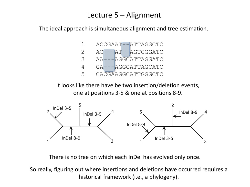
The ideal approach is simultaneous alignment and tree estimation.
1 ACCGAAT--ATTAGGCTC
2 AC---AT--AGTGGGATC
3 AA---AGGCATTAGGATC
4 GA---AGGCATTAGCATC
5 CACGAAGGCATTGGGCTC
So really, figuring out where insertions and deletions have occurred requires a
historical framework (i.e., a phylogeny).
There is no tree on which each InDel has evolved only once.
We need a way to evaluate alternative alignments
Goal: find the globally optimal combination of topology + alignment.
However, given that phylogenetic estimation from a single alignment is
a problem that is so computationally difficult as to require heuristic methods
(short cuts), simultaneous alignment is not at all feasible.
The most commonly use heuristic in MSA is progressive alignment.
Progressive Alignment
Overview
. Progressive alignment occurs in three steps.
1. A
pair-wise alignment
is generated for all (
n
2
-
n
)/2 pairs of sequences. A
pair-
wise distance
is estimated between each of the pairs (as above) and this is
entered into a distance matrix.
2. That distance matrix is subjected to an algorithmic tree building procedure (usually
UPGMA or NJ). This produces a
guide tree
.
3. This guide tree is used to align close sequences first and adds progressively more
distant sequences (from the guide tree), until all sequences are in the alignment.
Pair-wise alignments are conducted using Needleman-Wunsch (1970) algorithm
G A A T T C A G T T A (#1)
G G A T C G A (#2)
So L
1
= 11 and L
2
= 7
D
=
s + w g
S
i,j
= 1 if the nucleotide at position
i
of sequence #1 is the
same as that at position
j
of sequence #2
S
i,j
= 0 (mismatch score)
g
= 0 (gap penalty)
w
= 1 (gap weight)
Needleman-Wunsch
Generate a matrix with the two sequences on each axis (11x7)
We initialize it with a row and column of zeroes (gap cost).
Needleman-Wunsch
1
We fill in the entire matrix with the
M
i,j
for each cell.
Needleman-Wunsch
We trace back from the bottom right, following the path with the highest score.
D
= 6
All paths with a score of 6 represent optimal alignments.
All (
n
2
-
n
)/2 pairwise comparisons – Edit distances are used to form a pairwise matrix
This matrix is subjected to a quick tree-building algorithm (NJ or UPGMA).
4 GA---AGGCATTAGCATC
5 CACGAAGGCATTGGGCTC
Now, we have a series of positional homologies & we can begin phylogeny estimation.
Elaborations
:
A substitution matrix is used to calculate the scores for mismatches.
Biochemically similar amino acids v. radical changes (MAFFT).
Transitions cost less than transversions.
Gap costs can be elaborated so that there is a separate cost associated
with opening a new gap (GOP) vs. extending a gap (GEP).
Position-specific gap-open penalties are modified according to
residue type, using empirical observations in a set of alignments
based on 3D structures.
Each sequence can be weighted according to how different it is from
the other sequences. This accounts for the case where one specific
subfamily is over-represented in the data set.
The largest portion of time is invested in conducting all the pair-wise N-W
alignments to generate an initial distance matrix.
Use
k
-mer words (usually
k
= 6) to derive a distance.
F. Models in Alignment
One problem is that the final alignment is dependent on the parameters, and the
optimum parameter values depend on unknown processes of evolution
(i.e., insertion rate, deletion rate, and rates of various substitution types).
The Catch-22 is that we need a good tree to estimate these. This is because, as
discussed in the beginning of this lecture, alignment and historical information
are not independent of each other.
There have been two approaches:
One is iterative approaches (SATe II; Liu et al. 2012. Syst. Biol. 61:90)
Bundles MAFFT, Muscle, & RAxML
Also prunes subtrees in intermediate iterations.
BAliPhy:
Suchard M A , Redelings B D. 2006. Bioinformatics, 22:2047-2048.
Redelings. 2021. Bioinformatics, 37:3032-3034.
Simultaneous Alignment
This is a parametric approach that explores a vast state space:
ω
= (
Y
,
A
,τ,
T
,
Θ
,
Λ
).
Y – The data (unaligned sequences)
A – The alignment
τ
- The tree
T – Its branch lengths
Θ
– The substitution model
Λ
– The indel model
In the field of phylogenetics, the process of progressive alignment is crucial for aligning sequences and building evolutionary trees. This approach involves generating pairwise alignments, estimating distances, constructing guide trees, and aligning sequences progressively based on the tree. Needleman-Wunsch algorithm is used for pairwise alignments, facilitating the comparison and scoring of sequences. This method aids in finding the optimal combination of topology and alignment, essential for understanding evolutionary relationships.

Uploaded on Sep 07, 2024 | 0 Views
Download Presentation

Please find below an Image/Link to download the presentation.
The content on the website is provided AS IS for your information and personal use only. It may not be sold, licensed, or shared on other websites without obtaining consent from the author.If you encounter any issues during the download, it is possible that the publisher has removed the file from their server.
You are allowed to download the files provided on this website for personal or commercial use, subject to the condition that they are used lawfully. All files are the property of their respective owners.
The content on the website is provided AS IS for your information and personal use only. It may not be sold, licensed, or shared on other websites without obtaining consent from the author.
E N D
Presentation Transcript
Lecture 5 Alignment The ideal approach is simultaneous alignment and tree estimation. 1 ACCGAAT--ATTAGGCTC 2 AC---AT--AGTGGGATC 3 AA---AGGCATTAGGATC 4 GA---AGGCATTAGCATC 5 CACGAAGGCATTGGGCTC It looks like there have be two insertion/deletion events, one at positions 3-5 & one at positions 8-9. There is no tree on which each InDel has evolved only once. So really, figuring out where insertions and deletions have occurred requires a historical framework (i.e., a phylogeny).
We need a way to evaluate alternative alignments A simple score: D = s + w g Where s is the score for match/mismatch, g is a gap cost and w is a gap weight. Goal: find the globally optimal combination of topology + alignment. However, given that phylogenetic estimation from a single alignment is a problem that is so computationally difficult as to require heuristic methods (short cuts), simultaneous alignment is not at all feasible. The most commonly use heuristic in MSA is progressive alignment.
Progressive Alignment Overview. Progressive alignment occurs in three steps. 1. A pair-wise alignment is generated for all (n2-n)/2 pairs of sequences. A pair- wise distance is estimated between each of the pairs (as above) and this is entered into a distance matrix. 2. That distance matrix is subjected to an algorithmic tree building procedure (usually UPGMA or NJ). This produces a guide tree. 3. This guide tree is used to align close sequences first and adds progressively more distant sequences (from the guide tree), until all sequences are in the alignment.
Pair-wise alignments are conducted using Needleman-Wunsch (1970) algorithm G A A T T C A G T T A (#1) G G A T C G A (#2) So L1 = 11 and L2 = 7 D = s + w g Si,j= 1 if the nucleotide at position i of sequence #1 is the same as that at position j of sequence #2 Si,j= 0 (mismatch score) g = 0 (gap penalty) w = 1 (gap weight)
Needleman-Wunsch Generate a matrix with the two sequences on each axis (11x7) We initialize it with a row and column of zeroes (gap cost). G A A T T C A G T T A 0 0 0 0 0 0 0 0 0 0 0 0 G 0 G 0 A 0 T 0 C 0 G 0 A 0 The matrix is filled by finding the maximal score Mi,jfor each cell. Mi,j= Maximum value of: Mi-1, j-1+ Si,j(match/mismatch in the diagonal) 0+1=1 Mi,j-1 + wg (gap in sequence 1) 0+0=0 Mi-1, j + wg (gap in sequence 2) 0+0=0
Needleman-Wunsch G A A T T C A G T T A 0 0 0 0 0 0 0 0 0 0 0 0 G 0 G 0 A 0 T 0 C 0 G 0 A 0 1 We fill in the entire matrix with the Mi,j for each cell.
Needleman-Wunsch G A A T T C A G T T A 0 0 0 0 0 0 0 0 0 0 0 0 G 0 1 1 1 1 1 1 1 1 1 1 1 G 0 1 1 1 1 1 1 1 2 2 2 2 A 0 1 2 2 2 2 2 2 2 2 2 3 T 0 1 2 2 3 3 3 3 3 3 3 3 C 0 1 2 2 3 3 4 4 4 4 4 4 G 0 1 2 2 3 3 4 4 5 5 5 5 A 0 1 2 3 3 3 3 4 5 5 5 6 We trace back from the bottom right, following the path with the highest score. G | G - A | A A T | T T C | C A G | G T T A | A D = 6 G - - - - - All paths with a score of 6 represent optimal alignments. All (n2-n)/2 pairwise comparisons Edit distances are used to form a pairwise matrix
This matrix is subjected to a quick tree-building algorithm (NJ or UPGMA). Again, following the guide tree, we align sequence 3 to the fixed 1/2 alignment. 1 ACCGAAT--ATTAGGCTC 2 AC---AT--AGTGGGATC 3 AA---AGGCATTAGGATC 4 GA---AGGCATTAGCATC 5 CACGAAGGCATTGGGCTC Now, we have a series of positional homologies & we can begin phylogeny estimation.
Elaborations: A substitution matrix is used to calculate the scores for mismatches. Biochemically similar amino acids v. radical changes (MAFFT). Transitions cost less than transversions. Gap costs can be elaborated so that there is a separate cost associated with opening a new gap (GOP) vs. extending a gap (GEP). Each sequence can be weighted according to how different it is from the other sequences. This accounts for the case where one specific subfamily is over-represented in the data set. Position-specific gap-open penalties are modified according to residue type, using empirical observations in a set of alignments based on 3D structures.
The largest portion of time is invested in conducting all the pair-wise N-W alignments to generate an initial distance matrix. Use k-mer words (usually k = 6) to derive a distance. Muscle (Edgar. 2004. NAR.32:1792)
F. Models in Alignment One problem is that the final alignment is dependent on the parameters, and the optimum parameter values depend on unknown processes of evolution (i.e., insertion rate, deletion rate, and rates of various substitution types). The Catch-22 is that we need a good tree to estimate these. This is because, as discussed in the beginning of this lecture, alignment and historical information are not independent of each other. There have been two approaches: One is iterative approaches (SATe II; Liu et al. 2012. Syst. Biol. 61:90) Bundles MAFFT, Muscle, & RAxML Also prunes subtrees in intermediate iterations.
Simultaneous Alignment BAliPhy: Suchard M A , Redelings B D. 2006. Bioinformatics, 22:2047-2048. Redelings. 2021. Bioinformatics, 37:3032-3034. This is a parametric approach that explores a vast state space: = (Y,A, ,T, , ). Y The data (unaligned sequences) A The alignment The substitution model - The tree = s + w(g) The indel model T Its branch lengths