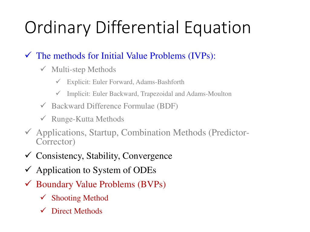
Ordinary Differential Equation

Ordinary Differential Equation The methods for Initial Value Problems (IVPs): Multi-step Methods Explicit: Euler Forward, Adams-Bashforth Implicit: Euler Backward, Trapezoidal and Adams-Moulton Backward Difference Formulae (BDF) Runge-Kutta Methods Applications, Startup, Combination Methods (Predictor- Corrector) Consistency, Stability, Convergence Application to System of ODEs Boundary Value Problems (BVPs) Shooting Method Direct Methods

ESO 208A: Computational Methods in Engineering Ordinary Differential Equation: Boundary Value Problems Abhas Singh Department of Civil Engineering IIT Kanpur Acknowledgements: Profs. Saumyen Guha and Shivam Tripathi (CE)

Boundary Value Problems A general 2nd Order Boundary Value Problem may be written as: ?2? ??2+ ? ?,? ?? ??+ ? ?,? = 0 ? ?,? subject to ? 0 = ?0, ? ? = ?? Higher order is also possible: ? + ??? + ? 1 ? 2 ? 0 = 0; ? 0 = 0; ? 0 = 5.0 = 0 ? 0,1 The last condition may be changed to: ? 1 = 1 Two approaches for solution: Convert to system of IVP (Shooting Method) Use difference approximations for the derivative (Direct method)

Shooting Method Consider the following equation: ? ? ? + ? ? ? + ? ? ? = ? ? ? 0,? subject to: ? 0 = ?, ? ? = ? Formulate the IVPs: Define: ? = ?, ? = ? ? = ? ? = ? ? ? ? ? ? ? ? +? ? ? ? ? ? ? 0 = ?, ? 0 =?,we have ? ? = ? Shooting Method Outline: Assume two initial values of v(0) and solve using any suitable method of IVPs to obtain the values of u(l) Use secant method to compute a new value of v(0) Iterate until ? ? ? < ?

Open Methods: Secant (Recap) Principle: Use a difference approximation for the slope or derivative in the Newton-Raphson method. This is equivalent to approximating the tangent with a secant. Problem: f(x) = 0, find a root x = such that f( ) = 0 f(x0) f(x1) f(x2) x0x1 x2 y = f(x) x3 5

Open Methods: Secant (Recap) Problem: f(x) = 0, find a root x = such that f( ) = 0 Initialize: choose two points x0 and x1 and evaluate f(x0) and f(x1) Approximation: ? ?? ? ?? ? ?? 1 Raphson , replace in Newton- ?? ?? 1 ?? ?? 1 ? ?? ? ?? 1 Iteration Formula: ??+1= ?? ? ?? ??+1 ?? ??+1 Stopping criteria: ? 6

Shooting Method Assume two initial values of v(0): v1(0) and v2(0) Solve using a suitable method of IVPs to obtain: u1(l) and u2(l) Use Secant method to compute a new value of v(0) as: ?20 ?10 ?2? ?1? ?30 = ?20 ?2? ? General Secant iteration scheme for the kth iteration is: ??0 ?? 10 ??? ?? 1? ??+10 = ??0 ??? ? Stopping Criterion: ?? ?? 1 ? ?? ? ?? 1 ??+1= ?? ? ?? ? ??? ? 100 <

Direct Method Let us consider the equation: ? ? ? + ? ? ? + ? ? ? = ? ? ? 0 = ? ; ? ? = ? 0 i i+1 n 1 2 i-1 n-1 Node Numbers:- x0 xi xi+1 xn x1 x2 xi-1 x-values:- xn-1 y-values:- y0 yi yi+1 yn y1 y2 yi-1 yn-1 Independent variable values at the grid points (known): ?0,?1,?2 ?? Dependent variable values at the grid points: ?0,?1,?2 ?? Known values of y at the grid points (from BCs): ?0= ?;??= ? Unknowns to be computed: ?1,?1,?2 ?? 1

Direct Method ? ? ? + ? ? ? + ? ? ? = ? ? ? 0 = ? ; ? ? = ? 0 i i+1 n 1 2 i-1 n-1 Node Numbers:- x0 xi xi+1 xn x1 x2 xi-1 x-values:- xn-1 y-values:- y0 yi yi+1 yn y1 y2 yi-1 yn-1 With 2nd order central difference approximation with grid length h, for any interior node i: ??+1 2??+ ?? 1 2 2 ??+1 ?? 1 ? ?? + ? ?? + ? ????= ? ??; ? = 1,..? 1 Rearranging: ? ?? 2 ? ?? ?? 1+ 2? ?? ? ?? 2 +? ?? + ? ?? ??+ ??+1= ? ?? 2 2 2

Direct Method 0 i i+1 n 1 2 i-1 n-1 Node Numbers:- x0 xi xi+1 xn x1 x2 xi-1 x-values:- xn-1 y-values:- y0 yi yi+1 yn y1 y2 yi-1 yn-1 ? ?? 2 Denote: ? ?? ?? 1+ 2? ?? ? ?? 2 +? ?? + ? ?? ??+ ??+1= ? ?? 2 2 2 ??=? ?? ? ?? ??= 2? ?? ??=? ?? +? ?? ; + ? ??; 2 2 2 2 2 Equations for the nodes: ? = 1: ?1?0+ ?1?1+ ?1?2= ? ?1 ? = 2: ?2?1+ ?2?2+ ?2?3= ? ?2 ? = ? 1: ?? 1?? 2+ ?? 1?? 1+ ?? 1??= ? ?? 1

Direct Method Equations for the nodes: ? = 1: ?1?0+ ?1?1+ ?1?2= ? ?1 ? = 2: ?2?1+ ?2?2+ ?2?3= ? ?2 ? = ? 1: ?? 1?? 2+ ?? 1?? 1+ ?? 1??= ? ?? 1 After putting the values of the BCs: ?0= ?;??= ? ? ?1 ?1? ? ?2 ? ?3 ? ?? 2 ? ?? 1 ?? 1? ?1 ?2 ?3 ?1 ?2 0 0 0 ?1 ?2 ?3 0 0 0 ?2 ?3 0 0 0 0 0 0 0 0 = ?? 2 ?? 1 ?? 2 0 ?? 2 ?? 1 ?? 2 ?? 1 What if in one of the BC, derivative is specified:? ? = ?or?? Two options: Backward Difference and Ghost Node Notice that ?? is now an unknown! Only last equation changes! = ?

Direct Method ? = ? 1: ?? 1?? 2+ ?? 1?? 1+ ?? 1??= ? ?? 1 The ?? is now an unknown The BC at i = n:? ? = ?or?? = ? Backward Difference: use the same order backward difference approximation as the order of approximation for the equation within the domain, in this case 2nd order, ?? 2 4?? 1+ 3?? 2 ??=2 3? +4 3?? 1 1 = ? 3?? 2 So the equation for i = n 1 becomes: ?? 1 ?? 1 3 ?? 2+ ?? 1+4?? 1 ?? 1= ? ?? 1 2?? 1 ? 3 3 Replace the last equation of the tri-diagonal matrix with this equation!

Direct Method Ghost Node: add a fictitious node (n + 1) beyond the boundary at a distance of h n 2 n + 1 n 1 n ? = ? 1: ?? 1?? 2+ ?? 1?? 1+ ?? 1??= ? ?? 1 We can now write an approximation of the original equation for node n ? = ?: ???? 1+ ????+ ????+1= ? ?? For the BC at i = n,? ? = ?or?? approximation: ??+1 ?? 1 = ?, use 2nd order central difference = ? ??+1= 2? + ?? 1 2 So the equation for i = n becomes: ??+ ???? 1+ ????= ? ?? 2? ?? Add this as the last equation of the tri-diagonal matrix. Size of the matrix increases by one!

Direct Method: Example Solve using Direct Method with 2nd Order central difference approximation with h = 0.25: ? + ? + ? = 0; ? [0,1]; ?(0) = ?(1) = 0 ??+1 2??+ ?? 1 0.252 + ??+ ??= 0 16?? 1 31??+ 16??+1= ?? 31?1+ 16?2 16?1 31?2+ 16?3= 0.5 16?2 31?3= 0.75 = 0.25 Thomas Algorithm: l d u b alpha s x -31 16 -0.25 -31.0000 -0.2500 0.0443 16 -31 16 -0.5 -22.7419 -0.6290 0.0702 16 -31 -0.75 -19.7433 -1.1926 0.0604

Direct Method: Example Compare the solutions obtained by Direct method and Shooting method with the Analytical solution: ? + ? + ? = 0; ? [0,1]; ?(0) = ?(1) = 0 Analytical Solution: ? =sin? sin1 ? x 0 y TRUE 0 Shooting 0 Error 0 Direct 0 Error 0 y0 y1 0.25 0.04401365 0.04460208 1.33691304 0.04427401 0.59154281 0.5 0.75 1 y2 y3 y4 0.06974696 0.07079153 1.49764749 0.0701559 0.58631705 0.06005617 0.06101881 1.60290267 0.06040305 0.57759244 0 2.7756E-17 0 0 0 Can you identify, why the solution with shooting method using 2nd order R-K does not give good solution for this problem?

Ordinary Differential Equation The methods for Initial Value Problems (IVPs): Multi-step Methods Explicit: Euler Forward, Adams-Bashforth Implicit: Euler Backward, Trapezoidal and Adams-Moulton Backward Difference Formulae (BDF) Runge-Kutta Methods Applications, Startup, Combination Methods (Predictor- Corrector) Consistency, Stability, Convergence Application to System of ODEs Boundary Value Problems (BVPs) Shooting Method Direct Methods

Applications: Summary of Concerns Accuracy of the higher order multi-step and BDF methods are affected if the starting values are used from the lower order methods. How to start these non-self starting algorithms? All implicit methods (multi-step and BDF) may involve solution of non-linear equations (if f contains a non-linear function of the dependent variable y) Is there a way to avoid this solution of non-linear equations? Numerical oscillations (instability) observed in some methods and not in some! Is there a way to predict and therefore, choose correct parameters for algorithm so that the numerical oscillations can be avoided? We will do Convergence Analysis!

ESO 208A: Computational Methods in Engineering Ordinary Differential Equation: Consistency, Stability, Convergence Abhas Singh Department of Civil Engineering IIT Kanpur Acknowledgements: Profs. Saumyen Guha and Shivam Tripathi (CE)

Numerical Methods for IVPs: Convergence Lax Equivalence Theorem: The numerical solution by a finite difference method converges to the true solution, if and only if, the method is both consistent and stable. Consistency: A finite difference method for an IVP is consistent if the global truncation error (GTE) is such that for any > 0, there exists a h( ) > 0 for which ??? < ?. This also means, lim 0??? = 0 A consistent numerical method is said to have an order of accuracy of p, if p is the largest positive integer such that ??? ? ? for 0 < ?, where K and h are constants. For all the methods derived so far, p 1, therefore, consistent!

Numerical Methods for IVPs: Consistency Consistency: This also means, ln ??? = ln ? + ?ln One can estimate the order of the method numerically. This is the same result of the Euler Forward method used for startup using different values of h. The absolute values of true errors were computed at h = 1.2

Numerical Methods for IVPs: Stability If numerical solutions for an IVP are obtained using a method with two sets of initial conditions ?0,?1,?2, ??and ?0,?1,?2, ??, the method is stable if there exists a constant K such that the following relation holds as h 0, ??+m ??+m ? max ?0 ?0, ?1 ?1, ?? ?? ? In true mathematical terminology, the method will be called zero stable. Consistency and zero stability are necessary conditions for convergence

Numerical Methods for IVPs: Stability Zero stability defines stability in asymptotic limit h 0 For application with h > 0, let us define an amplification factor ( ) ??+1 ?? = ? can be real or complex Condition of stability is satisfied if ? < 1 We need a model problem to assess and compare stability of various methods!

Stability: Model Problem Mathematical Problem: ?? ??= ? ?,? ? ?0 = ?0 ? 0 Since the solution starts from the fixed initial point (y0, t0) and expands to it s neighbourhood, let us explore the influence of function f(y, t) in this region: 2 ?2? ??2 ?? ??= ? ?0,?0 + ? ?0 ?? ?? ?? ?? ? ?0 2 + ? ?0 + ?0,?0 ?0,?0 ?0,?0 ?2? ???? 2 ?2? ??2 ? ?0 2 + ? ?0 ? ?0 + + ?0,?0 ?0,?0 Collecting only the linear terms: ?? ??= ? + ?? + ?? + ?? ??= ?? + ? ?

Stability: Model Problem ?? ??= ?? + ? ? Any approximate solution ? computed using a numerical method satisfies the approximate equation ? ? ??= ? ? + ? ? The error ( ) is defined as: ? = ? ?. We may write: ?? ??= ?? The function of the independent variable ? ? has no influence on the progression of error in the equation. Therefore the model problem for linear stability analysis is: ?? ??= ??; We may evaluate the analytical solution in a discrete grid ?0,?1,?2, ?? with a time step of h: ??= ?0??? ? = ?0??? ? 0 = ?0

Stability: Model Problem For general applicability to all types of functions or problems, we let to be complex: ? = ??+ ??? ??= ?0??? = ?0??? ??? ?? ? The analytical solution grows unbounded, i.e., ? > 1 if ?? > 0 irrespective of the value of ?? ?? We will now derive the stability regions of the numerical methods in the ?? vs. ?? - plane and compare that with the stability region of the analytical solution. ?? Stability region of the analytical solution of the model problem in the ?? vs. ?? - plane

Stability: Multi-Step Methods (explicit) Example Recall: The stability region (in the ?? vs. ?? - plane) of a numerical method is an open set C that contains the collection of those h for which ? < 1. Boundary of the region is often characterized by ? = 1. Since, is a function of h, is complex: ? = ??? ???= 1 ? < 1 < 1 Euler Forward: applying the method to the model problem, ?? ??= ??; ? 0 = ?0 ??= ???0 ??+1= ??+ ? ??= 1 + ?? + ??? ??= ??? 1 + ?? 2+ ?? 2< 1 ? = 1 + ?? + ??? < 1 For real : ??= 0; ??= ? (necessary for stability) 0 < <2 ?

Stability: Multi-Step Methods (explicit) Example Consider our problem: ?? ??= 2? + sin? For stability with Euler forward, h < 1 0 < <2 ?

Stability: Multi-Step Methods (explicit) Example For higher order methods, let s consider 3rd order Adams-Bashforth: Adams-Bashforth (3rd Order): applying the method to the model problem, 23 12??? 4 5 12??? 2 ??+1= ??+ 3??? 1+ ?3 ?2 23 12?2 4 ? = ?? + ??? = 3? +5 12 In order to plot the region, recall that the boundary of the region is characterized by ? = 1 or ? = ??? cos3? cos2? + ? sin3? sin2? 23 12cos2? 4 ?? + ??? = 3cos? +5 23 12sin2? 4 12+ ? 3sin? One can now easily compute ?? and ?? for ? 0,2? Let s compare the stability regions of all the explicit multi-step methods!

Stability: Multi-Step Methods (explicit) Example All explicit methods are conditionally stable. Consider our problem: ?? ??= 2? + sin? For stability with Adams-Bashforth (4th Order), h < 0.3/2 = 0.15

Stability: Multi-Step (Implicit) Euler Backward: applying the method to the model problem, ??+1 ?? 1 1 1 ??+1= ??+ ???+1 = ? = 1 ? = 1 ?? ??? = ?? 1 ?? ???? ? = tan 1 1 ?? 2+ ?? 2; ? = 1 ? 1 ?? 2+ ?? 2> 1 ? < 1 < 1 Euler Backward method is stable everywhere outside the circle! Homework: Stability region of the Trapezoidal Method!

Stability: Multi-Step Methods (implicit) Example For higher order methods, let s consider 3rd order Adams-Moulton: Adams-Moulton (3rd Order): applying the method to the model problem, 5 12???+1+2 1 12??? 1 ??+1= ??+ 3??? ?2 ? 3? 1 cos2? cos? + ? sin2? sin? 12cos2? +2 ?? + ??? = = 12?2+2 5 5 3cos? 1 12sin2? +2 5 12+ ? 3sin? 12 One can now easily compute ?? and ?? for ? 0,2? Let s compare the stability regions of all the implicit multi-step methods!

Stability: Multi-Step Methods (implicit) Example Euler backward method is unconditionally stable! (It is stable everywhere, where the analytical problem is also stable) Trapezoidal: find as homework! Adams-Moulton 3rd and 4th order methods are conditionally stable! Pay attention to the stability for purely imaginary !

Stability: BDF Methods Example 1storder BDF is the Euler Backward. For higher order methods, let s consider 3rd order BDF: BDF (3rd Order): applying the method to the model problem, 11 6??+1 3??+3 11 6 3 11 6 3cos? +3 2?? 1 1 3 2?2 3cos3? ? 3sin? 3 3?? 2= ? ??+1 1 ? = ?? + ??? = ?+ 3?3 2cos2? 1 2sin2? +1 = 3sin3? One can now easily compute ?? and ?? for ? 0,2? Let s compare the stability regions of all the BDF methods!

Stability: BDF Methods Example For all the BDFs: Stability Region is outside the enclosed region! For real , all the BDFs are unconditionally stable! One can use any h without having to worry about the stability! Useful for stiff equations!

Stability: Runge-Kutta Methods Example Let s consider 2nd order Runge-Kutta method for illustration: R-K Method (2nd Order): applying the method to the model problem, ??+1= ??+1 2?1, ?0= ? ??,??, ?1= ? ??+ ?0,??+ ??+1= ??+1 2 ? ??+ ??? 1 + ? +1 ?? One needs to find the roots of the polynomial to compute ?? and ?? for ? 0,2? 2?0+1 2 ???+1 2? 2=??+1 = ? = ???= cos? + ?sin?, ? 0, 2? For 2nd order R-K, the roots of the quadratic polynomial can be computed analytically! For the 3rd and 4th order R-K, the roots have to be computed numerically. Use complex version of Newton-Raphson. (Hint: roots are complex conjugates) Let s compare the stability regions of 2nd and 4th order R-K methods!

Stability: Runge-Kutta Methods Example 4th order R-K has very good stability properties ( h up to 2.78 on the real part and 2.83 on the imaginary part) The method is also stable for purely imaginary h Homework: For our problem, check the stability limits of the R-K methods!