Dynamic Function for Basal Area of Trees Derived from Differential Equation
Mathematical methods presented by Braun and Simmons are used to derive a dynamic function for the basal area of individual trees from a production-theoretically motivated autonomous differential equation. The differential equation and general dynamic function are described, highlighting the relationship between tree size, production efficiency, and basal area growth in forest settings.
Download Presentation

Please find below an Image/Link to download the presentation.
The content on the website is provided AS IS for your information and personal use only. It may not be sold, licensed, or shared on other websites without obtaining consent from the author.If you encounter any issues during the download, it is possible that the publisher has removed the file from their server.
You are allowed to download the files provided on this website for personal or commercial use, subject to the condition that they are used lawfully. All files are the property of their respective owners.
The content on the website is provided AS IS for your information and personal use only. It may not be sold, licensed, or shared on other websites without obtaining consent from the author.
E N D
Presentation Transcript
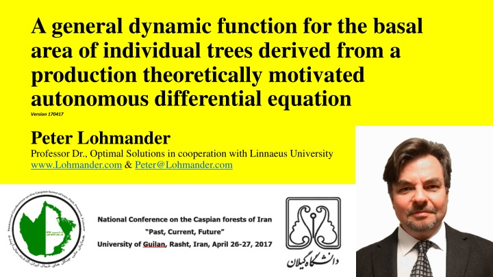
A general dynamic function for the basal area of individual trees derived from a production theoretically motivated autonomous differential equation Version 170417 Peter Lohmander Professor Dr., Optimal Solutions in cooperation with Linnaeus University www.Lohmander.com & Peter@Lohmander.com
A general dynamic function for the basal area of individual trees derived from a production theoretically motivated autonomous differential equation Peter Lohmander Abstract A general dynamic function for the basal area of individual trees has been derived from a production theoretically motivated autonomous differential equation. The differential equation is: dx dt ( ) = 1 1 , 0, 0,0 a x cx a c x c 2 + 1 1 x x c c + 0 a ct 1 e 0 = ( ) x t and the general dynamic function is: 2 + 1 1 x x c c 0 a ct 1 c e 0 Keywords: Dynamic function, differential equation, basal area, forest growth 2
Introduction The mathematical methods utilized in this paper are well presented by Braun (1983) and Simmons (1972). Now, fundamental biological production theory will suggest a relevant differential equation. We start with a small tree. 3
We start with a small tree. 4
Consider a stem segment, of height H of the tree. The stem segment is cylindrical with diameter D 1 D The leaves cover a cylinder with diameter 1 D D = 2 D 1, 1 2 H D 2 5
The sun light reaches the tree from the side. V is the volume of the stem segment. x is the basal area. = ( /4) Hx = 2 x V D 1 6
Volume increment is proportional to the photo synthesis level, P which in turn is proportional to the sun light projection area on the leaves, A = A HD 2 7
We may conclude that: dV dt dx dt = H P A D D x 2 1 Hence, dx dt dx dt= x , 0 a x a or 8
As the size of the tree increases, the production efficiency declines. Furthermore, the value of is often lower for large trees than for small trees. A relevant function considering this is: dx dt ( ) = 1 1 0, 0,0 a x cx a c x c 9
An illustration from the real world, using Scots pine (Pinus silvestris), from Sweden: 10
= 1.85 D m 3 = 1, 1 D D 2 For the small tree: 28.4 D D 3 1 ( ) D D 3 2 = 6.5 D cm 1 12
Let us investigate a large tree. 13
= 8.63 D m 3 = 1, 1 D D 2 For the large tree: 20.4 D D 3 1 ( ) D D 3 2 = 42.3 D cm 1 15
D D If 3 2 then is smaller for the large tree than for the small tree (in this case). A relevant function considering this is: dx dt ( ) = 1 1 0, 0,0 a x cx a c x c 16
Mathematical model development and analysis dx dt b a ( ) = = 1 1 , 0,0 a x cx c x c The parameters can be estimated via this linear reformulation: dx dt a b = 0.5 1.5 0, 0,0 ax bx a b x 17
dx dt b a ( ) = = 1 1 , 0,0 a x cx c x c 1 1 = dx adt ( ) x cx Integration gives 1 1 = + dx adt k ( ) 0 x cx 18
1 1 = + dx adt k ( ) 0 x cx ( ) ( ) + ln 1 ln 1 c x c x = + at k 0 c 19
( ) ( ) + ln 1 ln 1 c x c x = + at k 0 c Let us investigate the left hand side, called Z 1 c x 1 c x dZ dx c c = ( ) ( ) + 2 2 x x 1 1 c c 1 c x 1 c x dZ dx = ( ) ( ) + 2 1 2 1 x x 20
( ) ( 1 + ) 1 + 1 c x c x dZ dx = ( )( ) 2 1 x c x c x 1 1 dZ dx = ( ) x cx This confirmes that the integration was correct. 21
= + 1 1 c x c x c ln + at k 0 which leads to + 1 1 c x c x = + = ln cat k k ck 1 1 0 22
Let = = = , , y x g c h ga Then + 1 1 gy gy = + ln ht k 1 23
Let K = 1k e We get the simplified expression: + = 1 1 gy gy ht Ke which can be transformed to: ( ) + = ht 1 1 gy Ke gy or ( ) = ht ht 1 1 g Ke y Ke 24
ht 1 1 Ke Ke = y ( ) ht g + ht 1 ) ) 1 Ke = = y x which gives the desired equation ( ) ht 1 g Ke ( 2 + ht 1 Ke = ( ) x t ( 2 ht c Ke 25
Let us determine K = (0) x x We utilize the initial condition: ( ( c Ke Hence, ( 0 x 0 ) + 0 1 Ke ( ) = + = 1 1 x c K K x which leads to ) ) 0 0 0 1 = + 1 1 c K x c and finally 0 + 1 1 x x c c = 0 K 0 26
Now, we know how to determine K . Later, the sign and magnitude of K will be needed in the analysis. Do we know the sign of K ? ( 0 0 0 x c ) ( ) 1 0 + x c c 1 x Let us investigate the sign of 0 27
0x We assume that the value of makes sure that the increment is strictly positive. dx dt= ( ) 1 a x cx Then, we know that: 1 0 1 0 1 1 cx cx c x x c 0 0 0 0 K 0 As a result, we know that 28
Do we know the something about K ? + 1 1 = = 0 1 K x c 0 + 1 1 = = = = ( ) lim ( ) 1 K K 0 ( ) ( 1 ) + 2 1 dK d 1 dK d = 0 = ( ) 2 ( ) 2 1 K 1 With this information, we know that 29
0x Now, we may determine ( ) and the parameters. x t as an explicit function of ( ) 2 + ht 1 Ke + 1 1 x x c c = = = 0 ( ) x t K h a c ( ) 2 ht 1 c Ke 0 2 + 1 1 x x c c + 0 a ct 1 e 0 = ( ) x t 2 + 1 1 x x c c 0 a ct 1 c e 0 30
Now, the dynamic properties of ( ( c Ke ) 2 + ht 1 Ke = ( ) x t will be determined. ) 2 ht 1 ) ( 2 dx dt Khc ( )( ) ( ) ( 1 ) 2 2 = + + ht ht ht ht 1 1 1 Ke Ke Ke Ke ( ) 4 2 ht 1 c Ke 31
( )( ) + ht ht 2 1 1 Khc Ke Ke ( ) dx dt ( ) ( 1 ) = + ht ht 1 Ke Ke ( ) 4 2 ht 1 c ( Ke Ke ) ( ) . Hence, ( 2 ht 4 1 Khc Ke dx dt = ( ) 4 2 ht 1 c ) ( ) K dx dt 2 1 ht We already know that 1 0 Ke 0 As a result, we find that 32
( ) 2 + ht 1 d Ke 1 + ( ) 1 dt + ht 2 1 Ke hK 1 c ht Ke = = = = lim ( ) t h K x t ( ) ( ) 1 2 ht 2 1 c Ke hK ht 1 dc Ke 1 c 0 ht Ke 1 dt c 1 ( ) x t t , Hence, we know that, as monotonically converges to 33
How How does does the the function function work work? ? Below, parameter values representing the following case are used. Species: Maple (Acer velutinum) Initial diameter: 10 cm. Source: Hatami, Lohmander, Moayeri and Mohammadi Limaei (2017) Competition: No. 34
Basal Area (Square Centimeter) as a function of time, t (Years) 35
Basal Area (Square Centimeter) Time (Year) 36
Diameter (Centimeter) Time (Year) 38
Results A general dynamic function for the basal area of individual trees has been derived from a production theoretically motivated autonomous differential equation. The dynamic properties have been determined and monotone convergence has been proved. 39
Discussion The production theoretically motivated autonomous differential equation has recently been tested with regression analysis, using two sets of forest data from the Caspian forests. Detailed reports will soon be available. The parameters obtained the expected signs and the t-values indicated very high precision. The adjusted R2-values, the very high F-values and the lack of unexplained trends in the residual graphs, indicated a relevant model. The functional form has been found to work very well with empirical data from Iran and hopefully it will be possible to test it also on forest data from other regions of the world. 40
It is possible to use the model also under the influence of some forms of size dependent competition, via adjustments of the parameters ( , ) a b Further developements in this direction should be expected. Presently, different forest research projects with a strong focus on empirical investigations are active, in Sweden and in Iran. Hopefully, the derived analytical model will be useful in these projects. 41
Conclusions Differential equations can be very useful tools in forest management optimization. It is however important that they have theoretical and empirical support. Future efforts should be directed towards applications of the suggested and derived function within forest management problems in several regions of the world. 42
Acknowledgments The author is grateful to Associate Professor Soleiman Limaei who arranged several forest excursions and meetings Furthermore, he arranged meetings and cooperation interested PhD students with detailed forest data from the Caspian forests. Mohammadi in Iran. with seriously Thank you! 43
Acknowledgments Professor Linnaeus University in Sweden, coordinates a very interesting project on optimal continuous cover forestry and creates a very positive research environment. Johan Bergh, at Thank you! 44
A general dynamic function for the basal area of individual trees derived from a production theoretically motivated autonomous differential equation Version 170417 Peter Lohmander Professor Dr., Optimal Solutions in cooperation with Linnaeus University www.Lohmander.com & Peter@Lohmander.com
