Optimizing FIR Filters with Equiripple Algorithm
Explore how the Equiripple algorithm minimizes errors in FIR filter designs, achieving superior performance in frequency responses. Learn about filter specifications, design steps, and comparisons to other design methods.

Download Presentation

Please find below an Image/Link to download the presentation.
The content on the website is provided AS IS for your information and personal use only. It may not be sold, licensed, or shared on other websites without obtaining consent from the author. If you encounter any issues during the download, it is possible that the publisher has removed the file from their server.
You are allowed to download the files provided on this website for personal or commercial use, subject to the condition that they are used lawfully. All files are the property of their respective owners.
The content on the website is provided AS IS for your information and personal use only. It may not be sold, licensed, or shared on other websites without obtaining consent from the author.
E N D
Presentation Transcript
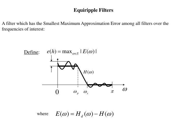
Equiripple Filters A filter which has the Smallest Maximum Approximation Error among all filters over the frequencies of interest: = ( ) max | ( | ) e h E Define: S ( ) H 0 p s = ( ) ( ) ( ) E H H where d
Fact: filters with the smallest maximum deviation from ideal characteristic are equiripple.. ( )| H | same ripple They are computed as follows: B=firpm(N,F,M) 0 F k ( ) 1 F=[F(1),F(2), ], M=[M(1), M(2), ]; Fs/2 F=1 corresponding to N = filter order. M F( ) 1 F( ) 3 F F( ) 4 F( ) 2
( ) = ( ) ( ) E H Hd Fact: the error is miminal in minmax sense, provided there exist L+2 frequencies 1 2 2 + ... , L E E E E i S | ( )| max | ( )| = i S = ( ) ( ) + 1 i i such that E( ) S 7 E( ) E( H( ) 3 5 11 E( ) E( ) E( ) 9 ) 1 E( ) Hd( ) 4 2 8 10 E( ) E( ) E( ) E( ) 6 E( ) 12 E( )
Example: see the same example we saw for the FIR filter with window. Recall the specs: 0 4 kHz kHz 5 1. Pass band 2. Stopband = 20 Fs kHz 3. Sampling Frequency Apply Remez Algorithm. You have to determine the filter order a priori, and let s choose the same order N=81: h=firpm(80,[0,0.4,0.5,1],[1,1,0,0]); (n ) h 0.5 0.4 0.3 The impulse response obtained is shown. 0.2 The frequency response is shown in the next slide, compared with the one we obtained by using the hamming window. Notice that the attenuation in the stopband is higher in the equiripple. 0.1 0 -0.1 0 20 40 60 80 100
( ) H 20 0 Equiripple (Remez Algorithm) -20 -40 -60 -80 -100 -120 0 0.5 1 1.5 2 2.5 3 3.5 20 ( ) H 0 Hamming window -20 -40 -60 -80 -100 -120 0 0.5 1 1.5 2 2.5 3 3.5
Frequency Response of the Non Ideal LPF ( )| H | 1 + 1 ripple 1 1 attenuation 2 f P STOP stop pass stop transition region LPF specified by: passband frequency P + 1 = 1 20 log RP dB passband ripple or 1 10 1 1 stopband frequency STOP = 20 log R dB stopband attenuation or 10 S 2 2
Best Design tool for FIR Filters: the Equiripple algorithm (or Remez). It minimizes the maximum error between the frequency responses of the ideal and actual filter. | ( )| H 1 1 + ripple 1 1 attenuation 2 / , 1,1,0,0 , 1 2 ( ) = , 0, , , , h firpm N w w 1 2 1 2 ] h = 0 [ h ],..., [ h N 2 N ( ) /w 20log ( ) ~ 1 10 22 2 1 /w 2 = 0 2 1 3 Linear Interpolation
Example: Low Pass Filter = Passband 0.4 P = 0.5 Stopband with attenuation 40dB 40 2 22 (0.5 0.4 ) S = = 37 Choose order N 20 ( )| H | 0 -20 Almost 40dB!!! -40 -60 -80 -100 -120 0 0.5 1 1.5 2 2.5 3 3.5
Example: Low Pass Filter Choose order N=40 > 37 10 ( )| H | 0 -10 -20 OK!!! -30 -40 -50 -60 -70 -80 0 0.5 1 1.5 2 2.5 3 3.5


")