Optimal Binary Search Trees: Expected Probes & Optimization
 undefined
M
A
/
C
S
S
E
4
7
3
D
a
y
2
8
O
p
t
i
m
a
l
B
S
T
s


OPTIMAL BINARY SEARCH TREES
Dynamic Programming Example
Warmup: Optimal linked list order
•
Suppose we have n distinct data items
x
1
, x
2
, …, x
n
in a linked list.
•
Also suppose that we know the probabilities p
1
,
p
2
, …, p
n
that each of these items is the item we'll
be searching for.
•
Questions we'll attempt to answer:
–
What is the expected number of probes before a
successful search completes?
–
How can we minimize this number?
–
What about an unsuccessful search?
Examples
•
p
i
= 1/n for each i.
–
What is the expected number of probes?
•
p
1
= ½, p
2
= ¼, …, p
n-1
= 1/2
n-1
, p
n
= 1/2
n-1
–
expected number of probes:
•
What if the same items are placed into the list in
the opposite order?
•
The next slide shows the evaluation of the last
two summations in Maple.
–
Good practice for you? prove them by induction
Calculations for previous slide
What if we don't know the probabilities?
1.
Sort the list so we can at least improve the average time for
unsuccessful search
2.
Self-organizing list:
–
Elements accessed more frequently move toward the front of the list;
elements accessed less frequently toward the rear.
–
Strategies:
•
Move ahead one position (exchange with previous element)
•
Exchange with first element
•
Move to Front (only efficient if the list is a linked list)
•
What we are actually likely to know is frequencies in previous
searches.
•
Our best estimate of the probabilities will be proportional to the
frequencies, so we can use frequencies instead of probabilities.
Optimal Binary Search Trees
•
Suppose we have n distinct data keys K
1
, K
2
, …, K
n
(in increasing order) that we wish to arrange into
a Binary Search Tree
•
Suppose we know the probabilities that a
successful search will end up at K
i
and the
probabilities that the key in an unsuccessful
search will be larger than K
i
and smaller than K
i+1
•
This time the expected number of probes for a
successful or unsuccessful search depends on the
shape of the tree and where the search ends up
–
Formula?
•
Guiding principle for optimization?
Example
•
For now we consider only successful searches,
with probabilities A(0.2), B(0.3), C(0.1), D(0.4).
•
What would be the worst-case arrangement
for the expected number of probes?
–
For simplicity, we'll multiply all of the probabilities
by 10 so we can deal with integers.
•
Try some other arrangements:
Opposite, Greedy, Better, Best?
•
Brute force: Try all of the possibilities and see
which is best. How many possibilities?
Aside: How many possible BST's
•
Given distinct keys K
1
< K
2
< … < K
n
, how many
different Binary Search Trees can be
constructed from these values?
•
Figure it out for n=2, 3, 4, 5
•
Write the recurrence relation
Aside: How many possible BST's
•
Given distinct keys K
1
< K
2
< … < K
n
, how many
different Binary Search Trees can be
constructed from these values?
•
Figure it out for n=2, 3, 4, 5
•
Write the recurrence relation
•
Solution is the
Catalan number
c(n)
•
Verify for n = 2, 3, 4, 5.
W
i
k
i
p
e
d
i
a
C
a
t
a
l
a
n
a
r
t
i
c
l
e
h
a
s
f
i
v
e
d
i
f
f
e
r
e
n
t
p
r
o
o
f
s
o
f
W
h
e
n
n
=
2
0
,
c
(
n
)
i
s
a
l
m
o
s
t
1
0
1
0
Optimal Binary Search Trees
•
Suppose we have n distinct data keys K
1
, K
2
, …,
K
n
(in increasing order) that we wish to arrange
into a Binary Search Tree
•
This time the expected number of probes for a
successful or unsuccessful search depends on
the shape of the tree and where the search
ends up
•
This discussion follows Reingold and Hansen,
Data Structures
.
An excerpt on optimal static
BSTS is posted on Moodle.
I use a
i
and b
i
where Reingold and Hansen use
α
i
and
β
i
.
Recap: Extended binary search tree
•
It's simplest to describe this
problem in terms of an
extended binary search tree
(EBST): a BST enhanced by
drawing "external nodes" in
place of all of the null pointers
in the original tree
•
Formally, an Extended Binary Tree (EBT) is either
–
an external node, or
–
an (internal) root node and two EBTs T
L
and T
R
•
In diagram, Circles = internal nodes, Squares = external
nodes
•
It's an alternative way of viewing a binary tree
•
The external nodes stand for places where an unsuccessful
search can end or where an element can be inserted
•
An EBT with n internal nodes has ___ external nodes
(We proved this by induction earlier in the term)
See Levitin:
page 183 [141]
What contributes to the expected
number of probes?
•
Frequencies, depth of node
•
For successful search, number of probes is
_______________ the depth of the
corresponding internal node
•
For unsuccessful, number of probes is
__________ the depth of the corresponding
external node
one more than
equal to
Optimal BST Notation
•
Keys are K
1
, K
2
, …, K
n
•
Let v be the value we are searching for
•
For i= 1, …,n, let a
i
be the probability that v is key K
i
•
For i= 1, …,n-1, let b
i
be the probability that K
i
< v < K
i+1
–
Similarly, let b
0
be the probability that v < K
1
,
and b
n
the probability that v > K
n
•
Note that
•
We can also just use
frequencies
instead of
probabilities
when finding the optimal tree (and divide by their sum to
get the probabilities if we ever need them). That is what
we will do in anexample.
•
Should we try exhaustive search of all
possible BSTs?
What not to measure
•
What about external path length and internal
path length?
•
These are too simple, because they do not take
into account the frequencies.
•
We need
weighted
path lengths
.
Weighted Path Length
•
If we divide this by
a
i
+
b
i
we get the expected
number of probes.
•
We can also define it recursively:
•
C(
) = 0. If T = , then
C(T) = C(T
L
) + C(T
R
) +
a
i
+
b
i
, where the
summations are over all a
i
and b
i
for nodes in T
•
It can be shown by induction that these two
definitions are equivalent
(a homework problem,).
T
L
T
R
N
o
t
e
:
y
0
,
…
,
y
n
a
r
e
t
h
e
e
x
t
e
r
n
a
l
n
o
d
e
s
o
f
t
h
e
t
r
e
e
Example
•
Frequencies of vowel occurrence in English
•
: A, E, I, O, U
•
a's: 32, 42, 26, 32, 12
•
b's: 0, 34, 38, 58, 95, 21
•
Draw a couple of trees (with E and I as roots),
and see which is best. (sum of a's and b's is
390).
Strategy
•
We want to minimize the weighted path length
•
Once we have chosen the root, the left and
right subtrees must themselves be optimal
EBSTs
•
We can build the tree from the bottom up,
keeping track of previously-computed values
Intermediate Quantities
•
Cost: Let C
ij
(for 0 ≤ i ≤ j ≤ n) be the cost of an
optimal tree (not necessarily unique) over the
frequencies b
i
, a
i+1
, b
i+1
, …a
j
, b
j
. Then
•
C
ii
= 0, and
•
This is true since the subtrees of an optimal
tree must be optimal
•
To simplify the computation, we define
•
W
ii
= b
i
, and W
ij
= W
i,j-1
+ a
j
+ b
j
for i<j.
•
Note that W
ij
= b
i
+ a
i+1
+ … + a
j
+ b
j
, and so
•
C
ii
= 0, and
•
Let R
ij
(root of best tree from i to j) be a value
of k that minimizes C
i,k-1
+ C
kj
in the above
formula
Code
Results
•
Constructed
by diagonals,
from main
diagonal
upward
•
What is the
optimal
tree?
H
o
w
t
o
c
o
n
s
t
r
u
c
t
t
h
e
o
p
t
i
m
a
l
t
r
e
e
?
A
n
a
l
y
s
i
s
o
f
t
h
e
a
l
g
o
r
i
t
h
m
?
•
Most frequent statement is the comparison
if C[i][k-1]+C[k][j] < C[i][opt-1]+C[opt][j]:
•
How many times
does it execute:
Running time
GREEDY ALGORITHMS
Do what seems best at the moment …
Greedy algorithms
•
Whenever a choice is to be made, pick the one that
seems optimal for the moment, without taking future
choices into consideration
–
Once each choice is made, it is irrevocable
•
For example, a greedy Scrabble player will simply
maximize her score for each turn, never saving any
“good” letters for possible better plays later
–
Doesn’t necessarily optimize score for entire game
•
Greedy works well for the "optimal linked list
with known search probabilities" problem, and
reasonably well for the "optimal BST" problem
–
But does not necessarily produce an optimal tree
Q7
Greedy Chess
•
Take a piece or pawn whenever you will not
lose a piece or pawn (or will lose one of lesser
value) on the next turn
•
Not a good strategy for this game either
Greedy Map Coloring
•
On a planar (i.e., 2D Euclidean) connected map,
choose a region and pick a color for that region
•
Repeat until all regions are colored:
–
Choose an uncolored region R that is adjacent
1
to at
least one colored region
•
If there are no such regions, let R be any uncolored region
–
Choose a color that is different than the colors of the
regions that are adjacent to R
–
Use a color that has already been used if possible
•
The result is a valid map coloring, not necessarily
with the minimum possible number of colors
1
T
w
o
r
e
g
i
o
n
s
a
r
e
a
d
j
a
c
e
n
t
i
f
t
h
e
y
h
a
v
e
a
c
o
m
m
o
n
e
d
g
e
Spanning Trees for a Graph
Minimal Spanning Tree (MST)
•
Suppose that we have a connected network G
(a graph whose edges are labeled by numbers,
which we call
weights
)
•
We want to find a tree T that
–
spans the graph (i.e. contains all nodes of G).
–
minimizes (among all spanning trees)
the sum of the weights of its edges.
•
Is this MST unique?
•
One approach: Generate all spanning trees and
determine which is minimum
•
Problems:
–
The number of trees grows exponentially with N
–
Not easy to generate
–
Finding a MST directly is simpler and faster
M
o
r
e
d
e
t
a
i
l
s
s
o
o
n
Huffman's algorithm
•
Goal: We have a message that co9ntains n
different alphabet symbols. Devise an
encoding for the symbols that minimizes the
total length of the message.
•
Principles: More frequent characters have
shorter codes. No code can be a prefix of
another.
•
Algorithm: Build a tree form which the codes
are derived. Repeatedly join the two lowest-
frequency trees into a new tree.
Q8-10
Concept of optimal binary search trees by understanding how probabilities impact successful and unsuccessful searches. Learn strategies to minimize expected probes and optimize search efficiency, including dynamic programming examples and self-organizing list techniques.

Download Presentation

Please find below an Image/Link to download the presentation.
The content on the website is provided AS IS for your information and personal use only. It may not be sold, licensed, or shared on other websites without obtaining consent from the author.If you encounter any issues during the download, it is possible that the publisher has removed the file from their server.
You are allowed to download the files provided on this website for personal or commercial use, subject to the condition that they are used lawfully. All files are the property of their respective owners.
The content on the website is provided AS IS for your information and personal use only. It may not be sold, licensed, or shared on other websites without obtaining consent from the author.
E N D
Presentation Transcript
MA/CSSE 473 Day 28 Optimal BSTs
Dynamic Programming Example OPTIMAL BINARY SEARCH TREES
Warmup: Optimal linked list order Suppose we have n distinct data items x1, x2, , xn in a linked list. Also suppose that we know the probabilities p1, p2, , pn that each of these items is the item we'll be searching for. Questions we'll attempt to answer: What is the expected number of probes before a successful search completes? How can we minimize this number? What about an unsuccessful search?
Examples pi = 1/n for each i. What is the expected number of probes? p1 = , p2= , , pn-1 = 1/2n-1, pn = 1/2n-1 expected number of probes: 1 = + n i 1 n n i n = 2 2 1 1 i 2 2 2 1 What if the same items are placed into the list in the opposite order? 1 2 = i 1 n n i + = + 1 n + 1 1 1 n i n 2 2 2 The next slide shows the evaluation of the last two summations in Maple. Good practice for you? prove them by induction
What if we don't know the probabilities? 1. Sort the list so we can at least improve the average time for unsuccessful search Self-organizing list: Elements accessed more frequently move toward the front of the list; elements accessed less frequently toward the rear. Strategies: Move ahead one position (exchange with previous element) Exchange with first element Move to Front (only efficient if the list is a linked list) What we are actually likely to know is frequencies in previous searches. Our best estimate of the probabilities will be proportional to the frequencies, so we can use frequencies instead of probabilities. 2.
Optimal Binary Search Trees Suppose we have n distinct data keys K1, K2, , Kn (in increasing order) that we wish to arrange into a Binary Search Tree Suppose we know the probabilities that a successful search will end up at Ki and the probabilities that the key in an unsuccessful search will be larger than Ki and smaller than Ki+1 This time the expected number of probes for a successful or unsuccessful search depends on the shape of the tree and where the search ends up Formula? Guiding principle for optimization?
Example For now we consider only successful searches, with probabilities A(0.2), B(0.3), C(0.1), D(0.4). What would be the worst-case arrangement for the expected number of probes? For simplicity, we'll multiply all of the probabilities by 10 so we can deal with integers. Try some other arrangements: Opposite, Greedy, Better, Best? Brute force: Try all of the possibilities and see which is best. How many possibilities?
Aside: How many possible BST's Given distinct keys K1 < K2< < Kn, how many different Binary Search Trees can be constructed from these values? Figure it out for n=2, 3, 4, 5 Write the recurrence relation
Aside: How many possible BST's Given distinct keys K1 < K2< < Kn, how many different Binary Search Trees can be constructed from these values? Figure it out for n=2, 3, 4, 5 Write the recurrence relation Solution is the Catalan number c(n) When n=20, c(n) is almost 1010 2 n + n n 1 + 2 ( )! + 4 n n k = = = = ( ) c n n 1 ( ! n 1 )! / 3 2 n n k n 2 k Verify for n = 2, 3, 4, 5. Wikipedia Catalan article has five different proofs of
Optimal Binary Search Trees Suppose we have n distinct data keys K1, K2, , Kn (in increasing order) that we wish to arrange into a Binary Search Tree This time the expected number of probes for a successful or unsuccessful search depends on the shape of the tree and where the search ends up This discussion follows Reingold and Hansen, Data Structures. An excerpt on optimal static BSTS is posted on Moodle. I use ai and bi where Reingold and Hansen use i and i .
Recap: Extended binary search tree It's simplest to describe this problem in terms of an extended binary search tree (EBST): a BST enhanced by drawing "external nodes" in place of all of the null pointers in the original tree Formally, an Extended Binary Tree (EBT) is either an external node, or an (internal) root node and two EBTs TL and TR In diagram, Circles = internal nodes, Squares = external nodes It's an alternative way of viewing a binary tree The external nodes stand for places where an unsuccessful search can end or where an element can be inserted An EBT with n internal nodes has ___ external nodes (We proved this by induction earlier in the term) See Levitin: page 183 [141]
What contributes to the expected number of probes? Frequencies, depth of node For successful search, number of probes is _______________ the depth of the corresponding internal node For unsuccessful, number of probes is __________ the depth of the corresponding external node one more than equal to
Optimal BST Notation Keys are K1, K2, , Kn Let v be the value we are searching for For i= 1, ,n, let ai be the probability that v is key Ki For i= 1, ,n-1, let bi be the probability that Ki < v < Ki+1 Similarly, let b0 be the probability that v < K1, and bn the probability that v > Kn Note that = = i i 1 0 n n + = 1 a b i i We can also just use frequencies instead of probabilities when finding the optimal tree (and divide by their sum to get the probabilities if we ever need them). That is what we will do in anexample. Should we try exhaustive search of all possible BSTs?
What not to measure What about external path length and internal path length? These are too simple, because they do not take into account the frequencies. We need weighted path lengths.
Weighted Path Length i i x depth a n n Note: y0, , yn are the external nodes of the tree = i = + + ( ) 1 [ ( ] ) [ ( ] ) i C T b depth y i = 1 0 i If we divide this by ai + bi we get the expected number of probes. We can also define it recursively: C( ) = 0. If T = , then TL TR C(T) = C(TL) + C(TR) + ai + bi , where the summations are over all ai and bi for nodes in T It can be shown by induction that these two definitions are equivalent (a homework problem,).
Example Frequencies of vowel occurrence in English : A, E, I, O, U a's: 32, 42, 26, 32, 12 b's: 0, 34, 38, 58, 95, 21 Draw a couple of trees (with E and I as roots), and see which is best. (sum of a's and b's is 390).
Strategy We want to minimize the weighted path length Once we have chosen the root, the left and right subtrees must themselves be optimal EBSTs We can build the tree from the bottom up, keeping track of previously-computed values
Intermediate Quantities Cost: Let Cij(for 0 i j n) be the cost of an optimal tree (not necessarily unique) over the frequencies bi, ai+1, bi+1, aj, bj. Then Cii = 0, and This is true since the subtrees of an optimal tree must be optimal To simplify the computation, we define Wii = bi, and Wij = Wi,j-1 + aj + bj for i<j. Note that Wij = bi + ai+1+ + aj + bj, and so Cii = 0, and Let Rij (root of best tree from i to j) be a value of k that minimizes Ci,k-1 + Ckj in the above formula j j = t = i t = + + + min C ( ) C C b a , 1 ij i k kj t t i k j + 1 i = + + min k i ( ) C W C C , 1 ij ij i k kj j
Results Constructed by diagonals, from main diagonal upward What is the optimal tree? How to construct the optimal tree? Analysis of the algorithm?
Running time Most frequent statement is the comparison if C[i][k-1]+C[k][j] < C[i][opt-1]+C[opt][j]: How many times does it execute: + n n d i d = = d i 1 0 1 = + 2 k i
Do what seems best at the moment GREEDY ALGORITHMS
Greedy algorithms Whenever a choice is to be made, pick the one that seems optimal for the moment, without taking future choices into consideration Once each choice is made, it is irrevocable For example, a greedy Scrabble player will simply maximize her score for each turn, never saving any good letters for possible better plays later Doesn t necessarily optimize score for entire game Greedy works well for the "optimal linked list with known search probabilities" problem, and reasonably well for the "optimal BST" problem But does not necessarily produce an optimal tree Q7
Greedy Chess Take a piece or pawn whenever you will not lose a piece or pawn (or will lose one of lesser value) on the next turn Not a good strategy for this game either
Greedy Map Coloring On a planar (i.e., 2D Euclidean) connected map, choose a region and pick a color for that region Repeat until all regions are colored: Choose an uncolored region R that is adjacent1 to at least one colored region If there are no such regions, let R be any uncolored region Choose a color that is different than the colors of the regions that are adjacent to R Use a color that has already been used if possible The result is a valid map coloring, not necessarily with the minimum possible number of colors 1 Two regions are adjacent if they have a common edge
Minimal Spanning Tree (MST) Suppose that we have a connected network G (a graph whose edges are labeled by numbers, which we call weights) We want to find a tree T that spans the graph (i.e. contains all nodes of G). minimizes (among all spanning trees) the sum of the weights of its edges. Is this MST unique? One approach: Generate all spanning trees and determine which is minimum Problems: The number of trees grows exponentially with N Not easy to generate Finding a MST directly is simpler and faster More details soon
Huffman's algorithm Goal: We have a message that co9ntains n different alphabet symbols. Devise an encoding for the symbols that minimizes the total length of the message. Principles: More frequent characters have shorter codes. No code can be a prefix of another. Algorithm: Build a tree form which the codes are derived. Repeatedly join the two lowest- frequency trees into a new tree. Q8-10


")