Numerical Integration in Numerical Methods
CISE301_Topic7
KFUPM
1
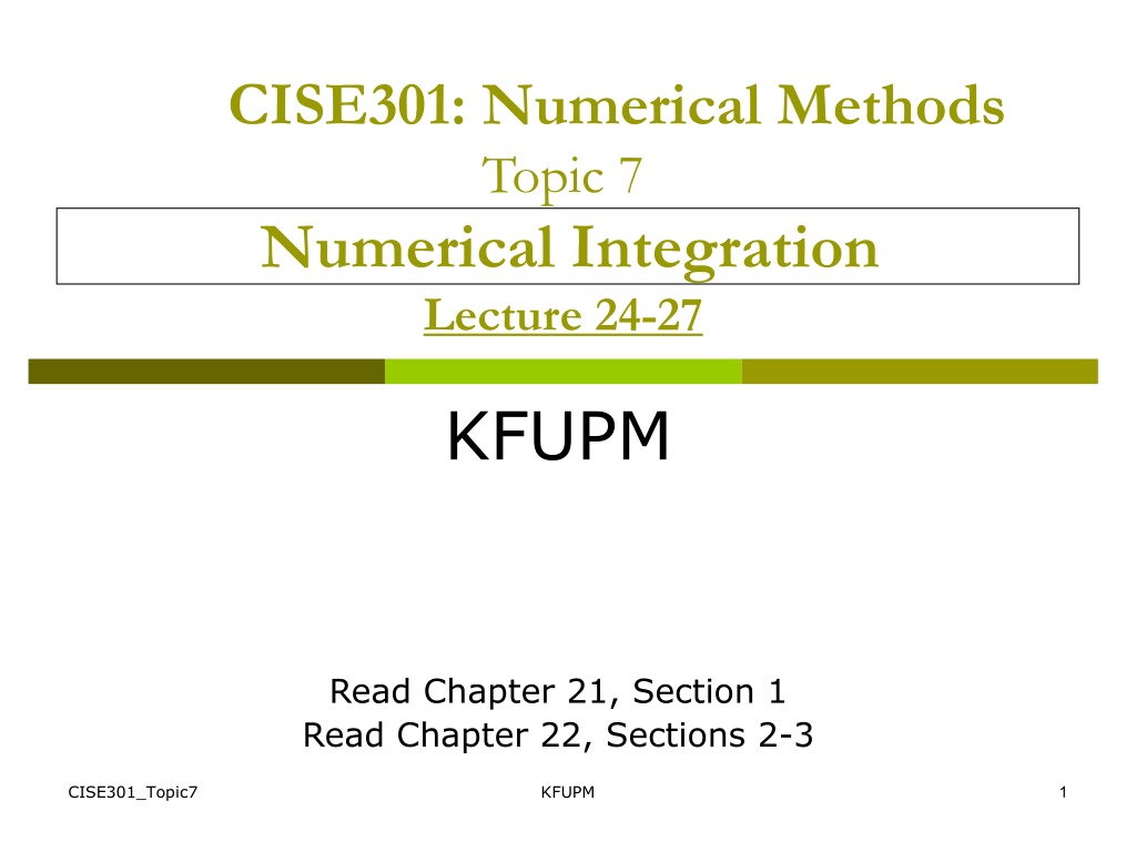
CISE301: Numerical Methods
Topic 7
Numerical Integration
Lecture 24-27
KFUPM
Read Chapter 21, Section 1
Read Chapter 22, Sections 2-3
CISE301_Topic7
KFUPM
2
L
ecture 24
Introduction to Numerical
Integration
Definitions
Upper and Lower Sums
Trapezoid Method (Newton-Cotes Methods)
Romberg Method
Gauss Quadrature
Examples
CISE301_Topic7
KFUPM
3
Integration
Integration
Indefinite Integrals
Indefinite Integrals of a
function are
functions
that differ from each
other by a constant.
Definite Integrals
Definite Integrals are
numbers.
CISE301_Topic7
KFUPM
4
Fundamental Theorem of Calculus
Fundamental Theorem of Calculus
CISE301_Topic7
KFUPM
5
The Area Under the Curve
The Area Under the Curve
One interpretation of the definite integral is:
Integral = area under the curve
a
b
f(x)
CISE301_Topic7
KFUPM
6
Upper and Lower Sums
Upper and Lower Sums
a
b
f(x)
The interval is divided into subintervals.
CISE301_Topic7
KFUPM
7
Upper and Lower Sums
Upper and Lower Sums
a
b
f(x)
CISE301_Topic7
KFUPM
8
Example
Example
CISE301_Topic7
KFUPM
9
Example
Example
CISE301_Topic7
KFUPM
10
Upper and Lower Sums
Upper and Lower Sums
•
Estimates based on Upper and Lower
Sums are easy to obtain for
monotonic
functions (
always increasing or always
decreasing
).
•
For non-monotonic functions, finding
maximum and minimum of the function
can be difficult and other methods can be
more attractive.
CISE301_Topic7
KFUPM
11
Newton-Cotes Methods
In
Newton-Cote Methods
, the function
is approximated by a
polynomial of
order
n
.
Computing the integral of a polynomial
is easy.
CISE301_Topic7
KFUPM
12
Newton-Cotes Methods
Trapezoid Method
(
First Order Polynomials are used
)
Simpson 1/3 Rule
(
Second Order Polynomials are used
)
CISE301_Topic7
KFUPM
13
L
ecture 25
Trapezoid Method
Derivation-One Interval
Multiple Application Rule
Estimating the Error
Recursive Trapezoid Method
Read 21.1
CISE301_Topic7
KFUPM
14
Trapezoid Method
Trapezoid Method
f(x)
CISE301_Topic7
KFUPM
15
Trapezoid Method
Derivation-One Interval
CISE301_Topic7
KFUPM
16
Trapezoid Method
Trapezoid Method
f(x)
CISE301_Topic7
KFUPM
17
Trapezoid Method
Trapezoid Method
Multiple Application Rule
Multiple Application Rule
a
b
f(x)
x
CISE301_Topic7
KFUPM
18
Trapezoid Method
Trapezoid Method
General Formula and Special Case
General Formula and Special Case
CISE301_Topic7
KFUPM
19
Example
Given a tabulated
values of the velocity of
an object.
Obtain an estimate of
the distance traveled in
the interval [0,3].
Distance = integral of the velocity
CISE301_Topic7
KFUPM
20
Example 1
Example 1
CISE301_Topic7
KFUPM
21
Estimating the Error
Estimating the Error
For Trapezoid Method
For Trapezoid Method
CISE301_Topic7
KFUPM
22
Error in estimating the integral
Error in estimating the integral
Theorem
Theorem
CISE301_Topic7
KFUPM
23
Example
Example
CISE301_Topic7
KFUPM
24
Example
Example
CISE301_Topic7
KFUPM
25
Example
Example
CISE301_Topic7
KFUPM
26
Recursive Trapezoid Method
Recursive Trapezoid Method
f(x)
CISE301_Topic7
KFUPM
27
Recursive Trapezoid Method
Recursive Trapezoid Method
f(x)
Based on previous estimate
Based on new point
Recall special
case of Trapezoid
Method!!
CISE301_Topic7
KFUPM
28
Recursive Trapezoid Method
Recursive Trapezoid Method
f(x)
Based on previous estimate
Based on new points
CISE301_Topic7
KFUPM
29
Recursive Trapezoid Method
Recursive Trapezoid Method
Formulas
Formulas
CISE301_Topic7
KFUPM
30
Recursive Trapezoid Method
Recursive Trapezoid Method
CISE301_Topic7
KFUPM
31
Advantages of Recursive Trapezoid
Recursive Trapezoid:
Gives the same answer as the standard
Trapezoid method.
Makes use of the available information to
reduce the computation time.
Useful if the number of iterations is not
known in advance.
CISE301_Topic7
KFUPM
32
L
ecture 26
Romberg Method
Motivation
Derivation of Romberg Method
Romberg Method
Example
When to stop?
Read 22.2
CISE301_Topic7
KFUPM
33
Motivation for Romberg Method
Motivation for Romberg Method
Trapezoid formula with an interval
h
gives an
error of the order
O(h
2
).
We can combine two Trapezoid estimates with
intervals 2h and h to get a better estimate.
CISE301_Topic7
KFUPM
34
Romberg Method
Romberg Method
First column is obtained
using Trapezoid Method
The other elements
are obtained using
the Romberg Method
CISE301_Topic7
KFUPM
35
First Column
First Column
Recursive Trapezoid Method
Recursive Trapezoid Method
CISE301_Topic7
KFUPM
36
Derivation of Romberg Method
Derivation of Romberg Method
CISE301_Topic7
KFUPM
37
Romberg Method
Romberg Method
CISE301_Topic7
KFUPM
38
Property of Romberg Method
Property of Romberg Method
Error Level
CISE301_Topic7
KFUPM
39
Example 1
Example 1
CISE301_Topic7
KFUPM
40
Example 1 (cont.)
Example 1 (cont.)
CISE301_Topic7
KFUPM
41
When do we stop?
When do we stop?
CISE301_Topic7
KFUPM
42
L
ecture 27
Gauss Quadrature
Motivation
General integration formula
Read 22.4
CISE301_Topic7
KFUPM
43
Motivation
Motivation
Figure 22.6, p. 641
Large overall
error
Smaller
overall error
CISE301_Topic7
KFUPM
44
Motivation (Contd.)
Motivation (Contd.)
CISE301_Topic7
KFUPM
45
General Integration Formula
General Integration Formula
CISE301_Topic7
KFUPM
46
Question
Question
What is the best way to choose the nodes
and the weights?
CISE301_Topic7
KFUPM
47
Question (Contd.)
Question (Contd.)
•
From previous figure, the integration is
exact
for a
polynomial of order
3 with 4 points (
c
0
,
c
1
,
x
0
, and
x
1
)
•
Integrate each of the four
f
(
x
)
polynomials ( )
•
Solve for
c
0
,
c
1
,
x
0
, and
x
1
c
0
=
c
1
= 1,
x
0
= ,
x
1
=
CISE301_Topic7
KFUPM
48
Gauss–Legendre Quadrature
(generalization of previous example)
A
n
n
-
p
o
i
n
t
G
a
u
s
s
-
L
e
g
e
n
d
r
e
Q
u
a
d
r
a
t
u
r
e
r
u
l
e
i
s
c
o
n
s
t
r
u
c
t
e
d
t
o
y
i
e
l
d
a
n
e
x
a
c
t
r
e
s
u
l
t
f
o
r
p
o
l
y
n
o
m
i
a
l
s
o
f
d
e
g
r
e
e
2
n
−
1
o
r
l
e
s
s
b
y
a
s
u
i
t
a
b
l
e
c
h
o
i
c
e
o
f
t
h
e
p
o
i
n
t
s
x
i
a
n
d
w
e
i
g
h
t
s
c
i
f
o
r
i
=
1
,
.
.
.
,
n
.
Source:
https://en.wikipedia.org/wiki/Gaussian_quadrature
and
https://en.wikipedia.org/wiki/Legendre_polynomials
CISE301_Topic7
KFUPM
49
Gauss–Legendre Quadrature
Gauss–Legendre Quadrature
See more in Table 22.1 (page 646)
See more in Table 22.1 (page 646)
CISE301_Topic7
KFUPM
50
Error Analysis for Gauss Quadrature
Error Analysis for Gauss Quadrature
CISE301_Topic7
KFUPM
51
Example
Example
CISE301_Topic7
KFUPM
52
Example
Example
CISE301_Topic7
KFUPM
53
Improper Integrals
Improper Integrals
This lecture covers the fundamentals of numerical integration, including upper and lower sums, trapezoid method, Romberg method, Gauss quadrature, definite and indefinite integrals, the fundamental theorem of calculus, and the area under the curve. The concepts are explained with examples and calculations to help understand the numerical methods for integration. Various methods and interpretations related to numerical integration in mathematics are discussed in detail.

Download Presentation

Please find below an Image/Link to download the presentation.
The content on the website is provided AS IS for your information and personal use only. It may not be sold, licensed, or shared on other websites without obtaining consent from the author.If you encounter any issues during the download, it is possible that the publisher has removed the file from their server.
You are allowed to download the files provided on this website for personal or commercial use, subject to the condition that they are used lawfully. All files are the property of their respective owners.
The content on the website is provided AS IS for your information and personal use only. It may not be sold, licensed, or shared on other websites without obtaining consent from the author.
E N D
Presentation Transcript
CISE301: Numerical Methods Topic 7 Numerical Integration Lecture 24-27 KFUPM Read Chapter 21, Section 1 Read Chapter 22, Sections 2-3 CISE301_Topic7 KFUPM 1
Lecture 24 Introduction to Numerical Integration Definitions Upper and Lower Sums Trapezoid Method (Newton-Cotes Methods) Romberg Method Gauss Quadrature Examples CISE301_Topic7 KFUPM 2
Integration Definite Integrals Indefinite Integrals 1 1 2 2 1 x 2 x = + = = x dx c xdx 2 2 0 0 Indefinite Integrals of a function are functions that differ from each other by a constant. Definite Integrals are numbers. CISE301_Topic7 KFUPM 3
Fundamental Theorem of Calculus If is continuous on an interval is antiderivative F , f [a,b] F = of (i.e., ' ( ) f ( ) ) f x x b = F(b) F(a) f(x)dx a 2 x There is no antiderivat for: i e v e b 2 x Noclosed form solution fo r: e dx a CISE301_Topic7 KFUPM 4
The Area Under the Curve One interpretation of the definite integral is: Integral = area under the curve f(x) b af(x)dx = Area a b CISE301_Topic7 KFUPM 5
Upper and Lower Sums The interval is divided into subintervals. = = = ... Partition P a x x x x b 0 1 2 n Define = min ( : ) m f x ( x x x f(x) + 1 i i x i x = max : ) M f x x + 1 i i i 1 n ( ) = ( , ) Lower sum L f P m x x + 1 i i i = 0 i 1 n ( ) = ( , ) Upper sum U f P M x x x x x x + 1 i i i 0 1 2 3 = 0 i a b CISE301_Topic7 KFUPM 6
Upper and Lower Sums 1 n ( ) = ( , ) Lower sum L f P m x x + 1 i i i = 0 i 1 n ( ) f(x) = ( , ) Upper sum U f P M x x + 1 i i i = 0 i + L U = Estimate of the integral 2 U L Error 2 x x x x 0 1 2 3 a b CISE301_Topic7 KFUPM 7
Example 1 2 x dx 0 1 2 3 = : , 0 , , 1 , Partition P 4 4 4 = 4 ( four equal intervals ) n 1 1 9 = = = = , 0 , , m m m m 0 1 2 3 16 4 16 1 1 9 = = = = , , , 1 M M M M 0 1 2 3 16 4 16 1 1 1 3 = = 0 1 3 , 2 , 1 , 0 x x for i + 1 i i 4 2 4 4 CISE301_Topic7 KFUPM 8
Example 1 n ( ) i = ( , ) Lower sum L f P m x x + 1 i i i = 0 1 1 1 9 14 = + + + = ( , ) 0 L f P 4 16 4 16 64 1 n ( ) i = ( , ) Upper sum U f P M x x + 1 i i i = 0 1 1 1 9 30 = + + + = ( , ) 1 U f P 4 16 4 16 64 1 30 14 11 = + = Estimate of the integral 2 64 64 32 1 30 14 1 = Error 2 64 64 8 1 1 3 0 1 4 2 4 CISE301_Topic7 KFUPM 9
Upper and Lower Sums Estimates based on Upper and Lower Sums are easy to obtain for monotonic functions (always increasing or always decreasing). For non-monotonic functions, finding maximum and minimum of the function can be difficult and other methods can be more attractive. CISE301_Topic7 KFUPM 10
Newton-Cotes Methods In Newton-Cote Methods, the function is approximated by a polynomial of order n. Computing the integral of a polynomial is easy. ( 0 1 ( ) a a ) b b + + + n ... f x dx a a x a x dx n + + + 2 2 1 1 n n ( ) ( ) b a b a b + + + ( ) f x dx ( a b a ) ... a a 0 1 n 2 1 n a CISE301_Topic7 KFUPM 11
Newton-Cotes Methods Trapezoid Method (First Order Polynomials are used) b b ( ) + ( ) f x dx a a x dx 0 1 a a Simpson 1/3 Rule (Second Order Polynomials are used) ( a a ) b b 2 + + ( ) f x dx a a x a x dx 0 1 2 CISE301_Topic7 KFUPM 12
Lecture 25 Trapezoid Method Derivation-One Interval Multiple Application Rule Estimating the Error Recursive Trapezoid Method Read 21.1 CISE301_Topic7 KFUPM 13
Trapezoid Method b = ( ) I f x dx ( ) ( ) f b f a a + ( ) ( ) f a x a b a ( ) ( ) f b f a b + ( ) ( ) I f a x a dx b a a f(x) b ( ) ( ) f b f a = ( ) f a a x b a a b 2 ( ) ( ) f b f a x + 2 b a a a b + ( ) ( ) f b f a ( ) = b a 2 CISE301_Topic7 KFUPM 14
Trapezoid Method Derivation-One Interval ( ) ( ) f b f a b b = + ( ) ( ) ( ) I f x dx f a x a dx b a a a ( ) ( ) ( ) ( ) f b f a f b f a b + ( ) I f a a x dx b a b a a b b 2 ( ) ( ) ( ) ( ) f b f a f b f a x = + ( ) f a a x 2 b a b a a a ( ) ( ) ( ) b ( ) f b f a f b f a ( ) = + 2 2 ( ) ( ) f a a b a b a ( 2 ) b a a + ( ) ( ) f b f a ( ) = b a 2 CISE301_Topic7 KFUPM 15
Trapezoid Method f(x) (b ) f (a ) f b a ( ) ) b = + ( ) ( Area f a f 2 a b CISE301_Topic7 KFUPM 16
Trapezoid Method Multiple Application Rule + ( ) ( ) f x f x ( ) = 2 1 Area x x 2 1 2 f(x) The interval [a, b] is partitione = a into d x segments n = ... a x x x b 0 1 2 n b = ( ) sum of the areas f x dx of the trapezoid s x x x x x 0 1 2 3 a b CISE301_Topic7 KFUPM 17
Trapezoid Method General Formula and Special Case If a the x = interval x is divided into b segments n (not necessaril equal) y = ... x x 0 1 2 n 1 1 n = ( )( ) ) i x b + ( ) ( ) ( f x dx x x f x f + + 1 1 i i i 2 a 0 i Special Case (Equalliy spaced base points) for all i i x x h i + = 1 1 2 1 n b + + ( ) f x dx ( ) f x ( ) ( ) f x h f x 0 n i a = 1 i CISE301_Topic7 KFUPM 18
Example Given a tabulated values of the velocity of an object. Time (s) 0.0 1.0 2.0 3.0 Velocity (m/s) 0.0 10 12 14 Obtain an estimate of the distance traveled in the interval [0,3]. Distance = integral of the velocity Distance 3 = ( ) V t dt 0 CISE301_Topic7 KFUPM 19
Example 1 The interval divided is Time (s) 0.0 1.0 2.0 3.0 into 3 subinterva ls Velocity (m/s) 0.0 10 12 14 3 , 2 , 1 , 0 are Base points Trapezoid Method = = 1 h x x + 1 i i 1 1 n ( ) = i = + + ( ) ( ) ( ) T h f x f x f x 0 i n 2 1 1 = + + + = Distance 1 (10 12) 0 ( 2 14 ) 29 CISE301_Topic7 KFUPM 20
Estimating the Error For Trapezoid Method How many equally spaced intervals are 0 needed compute to sin( ) x dx decimal 5 to digit accuracy ? CISE301_Topic7 KFUPM 21
Error in estimating the integral Theorem is ) ( ' ' : Assumption x f continuous on = [a,b] Equal intervals (width ) h Theorem : If Trapezoid Method is used to b approximat e ( ) then f x dx a b a = 2 ' ' ( ) Error h f where [a,b] 12 b a 2 max [ a x ( ' ' ) Error h f x 12 , ] b CISE301_Topic7 KFUPM 22
Example 1 5 sin( ) , error 10 x dx find h so that 2 0 b a 2 max = ( ' ' ) Error h f x 12 [ , cos( ] x a b = = = ; ; 0 ( ' ) ); ( ' ' ) sin( ) b a f x x f x x 1 2 5 ( ' ' ) 1 10 f x Error h 12 2 6 2 5 10 h CISE301_Topic7 KFUPM 23
Example x 1.0 1.5 2.0 2.5 3.0 f(x) 2.1 3.2 3.4 2.8 2.7 3 Use Trapezoid method compute to : ( ) f x dx 1 1 1 n ( )( ) = i = + ( , ) ( ) ( ) Trapezoid T f P x x f x f x + + 1 1 i i i i 2 x 0 = : for all , Special Case h x i + 1 i i 1 1 n ( ) = i = + + ( , ) ( ) ( ) ( ) T f P h f x f x f x 0 i n 2 1 CISE301_Topic7 KFUPM 24
Example x 1.0 1.5 2.0 2.5 3.0 f(x) 2.1 3.2 3.4 2.8 2.7 1 n 1 3 ( ) = i + + ( ) ( ) ( ) ( ) f x dx h f x f x f x 0 i n 2 1 1 1 ( 1 . 2 ) = 4 . 3 + 8 . 2 + + 7 . 2 + 5 . 0 2 . 3 2 9 . 5 = CISE301_Topic7 KFUPM 25
Recursive Trapezoid Method Estimate based on one interval : f(x) = h b a b a ( ) ) b = + ) 0 , 0 ( R ( ) ( f a f 2 + a a h CISE301_Topic7 KFUPM 26
Recursive Trapezoid Method Estimate based on intervals 2 : f(x) Recall special case of Trapezoid Method!! b a = h 2 1 b a ( ) = + + + ) 0 , 1 ( R ( ) ( ) ( ) f a h f a f b 2 2 1 ) h = + + ) 0 , 1 ( R ) 0 , 0 ( R ( h f a 2 + + 2 a a h a h Based on previous estimate Based on new point CISE301_Topic7 KFUPM 27
Recursive Trapezoid Method f(x) b a = h 4 b a = + + + + + ) 0 , 2 ( R ( ) ( 2 ) ( 3 ) f a h f a h f a h 4 1 ( ) + + ( ) ( ) f a f b 2 1 ) h = + + + + ) 0 , 2 ( R ) 0 , 1 ( R ( ) ( 3 h f a h f a 2 + + 2 4 a a h a h Based on previous estimate Based on new points CISE301_Topic7 KFUPM 28
Recursive Trapezoid Method Formulas b a = + ) 0 , 0 ( R ( ) ( ) f a f b 2 ) 1 (2 = n 1 ( ) = ) 0 , 1 + 2 ( + ) 1 ( ) 0 , ( R n R n h f a k h 2 1 k b a = h n 2 CISE301_Topic7 KFUPM 29
Recursive Trapezoid Method 2 b a = = + , ) 0 , 0 ( R ( ) ( ) h b a f a f b 2 1 1 b a ( ) = k = = + + , ) 0 , 1 ( R ) 0 , 0 ( R 2 ( ) 1 h h f a k h 2 1 2 2 1 b a ( ) = k = = + + , ) 0 , 2 ( R ) 0 , 1 ( R 2 ( ) 1 h h f a k h 2 2 1 2 2 2 1 b a ( ) = k = = + + , ) 0 , 3 ( R ) 0 , 2 ( R 2 ( ) 1 h h f a k h 3 2 1 .......... ........ ) 1 ( n 2 2 1 b a ( ) = k = = + + , ( ) 0 , n ( ) 0 , 1 2 ( ) 1 h R R n h f a k h n 2 1 CISE301_Topic7 KFUPM 30
Advantages of Recursive Trapezoid Recursive Trapezoid: Gives the same answer as the standard Trapezoid method. Makes use of the available information to reduce the computation time. Useful if the number of iterations is not known in advance. CISE301_Topic7 KFUPM 31
Lecture 26 Romberg Method Motivation Derivation of Romberg Method Romberg Method Example When to stop? Read 22.2 CISE301_Topic7 KFUPM 32
Motivation for Romberg Method Trapezoid formula with an interval h gives an error of the order O(h2). We can combine two Trapezoid estimates with intervals 2h and h to get a better estimate. CISE301_Topic7 KFUPM 33
Romberg Method Estimates using Trapezoid method with intervals of size , 2 , 4 ,8 ,... h h h h b are combined to improve the approximation of ( ) f x dx a R(0,0) First column is obtained using Trapezoid Method R(1,0) R(1,1) R(2,0) R(2,1) R(2,2) R(3,0) R(3,1) R(3,2) R(3,3) The other elements are obtained using the Romberg Method CISE301_Topic7 KFUPM 34
First Column Recursive Trapezoid Method b a = + ) 0 , 0 ( R ( ) ( ) f a f b 2 ) 1 (2 = n 1 ( ) = ) 0 , 1 + 2 ( + ) 1 ( ) 0 , ( R n R n h f a k h 2 1 k b a = h n 2 CISE301_Topic7 KFUPM 35
Derivation of Romberg Method n b a b = ) 0 , 1 + = 2 ( ) ( ( ) Trapezoid method f x dx R n O h with h 1 2 a b = ) 0 , 1 + + + + 2 4 6 ( ) ( ... ( ) 1 f x dx R n a h a h a h eq 2 4 6 a More accurate estimate obtained is by R(n,0) 1 1 1 b eq = + + + + 2 4 6 ( ) ( ) 0 , n ... ( ) 2 f x dx R a h a h a h eq 2 4 6 4 16 64 a 1 4 * 2 eq gives 1 b = + ) 0 , 1 + + + 4 6 ( ) ( ) 0 , n ( ) 0 , n ( ... f x dx R R R n b h b h 4 6 3 a CISE301_Topic7 KFUPM 36
Romberg Method b a R(0,0) R(1,0) = + ) 0 , 0 ( R ( ) ( ) f a f b 2 R(1,1) R(2,0) R(2,1) R(2,2) b a = , h R(3,0) R(3,1) R(3,2) R(3,3) n 2 ) 1 (2 = k n 1 ( ) = ) 0 , 1 + 2 ( + ) 1 ( ) 0 , n ( R R n h f a k h 2 1 1 = ) 1 + ) 1 , 1 ) 1 ( , ) ( , ( , ( R n m R n m R n m R n m m 4 m 1 , 1 1 for n CISE301_Topic7 KFUPM 37
Property of Romberg Method R(0,0) R(1,0) R(1,1) R(2,0) R(2,1) R(2,2) R(3,0) R(3,1) R(3,2) R(3,3) Theorem b a 2 + m = + 2 ( ) ( , ) ( ) f x dx R n m O h 2 4 6 8 ( ) ( ) ( ) ( ) O h O h O h O h Error Level CISE301_Topic7 KFUPM 38
Example 1 1 2 Compute x dx 0.5 3/8 1/3 0 1 b a = = + = + = , 1 ) 0 , 0 ( R ( ) ( ) 0 1 5 . 0 h f a f b 2 2 1 1 1 1 1 1 3 = = + + = + = , ) 0 , 1 ( R ) 0 , 0 ( R ( ( )) h h f a h 2 2 2 2 2 4 8 1 = ) 1 + ) 1 , 1 ) 1 ( , ) ( , ( , ( R n m R n m R n m R n m m 4 m 1 , 1 1 for n 1 3 1 3 1 1 = + = + = ) 1 , 1 ( R ) 0 , 1 ( R ) 0 , 1 ( R ) 0 , 0 ( R 1 8 3 8 2 3 4 1 CISE301_Topic7 KFUPM 39
0.5 Example 1 (cont.) 3/8 1/3 11/32 1/3 1/3 1 4 1 2 1 3 2 8 1 4 16 1 9 11 32 = = + + + + = + + = , (2,0) (1,0) ( ( h f a ) ( 3 )) h h R R h f a 16 1 = + ( , ) R n m ( , 1) ( , 1) ( 1, 1) R n m R n m R n m m 4 1 1 11 32 1 3 1 11 3 32 1 1 15 3 3 8 1 3 = + = + = (2,1) (2,0) (2,0) (1,0) R R R R 1 4 1 1 1 3 1 3 = + = + = (2,2) (2,1) (2,1) (1,1) R R R R 2 4 1 CISE301_Topic7 KFUPM 40
When do we stop? STOP if ) 1 , 1 ) 1 ( , ( R n m R n m or After a given number of steps, for example, STOP R(4,4) at CISE301_Topic7 KFUPM 41
Lecture 27 Gauss Quadrature Motivation General integration formula Read 22.4 CISE301_Topic7 KFUPM 42
Motivation Large overall error Figure 22.6, p. 641 Smaller overall error CISE301_Topic7 KFUPM 43
Motivation (Contd.) Trapezoid Method: 1 2 1 n b ( ) = + + ( ) f x dx ( ) f x ( ) f x ( ) h f x 0 i n a = 1 i It can be expressed as: n b = ( ) f x dx ( ) c f x i i a = 0 i = = 1,2,..., 0 and n 1 h i i n = where c i 0.5 h CISE301_Topic7 KFUPM 44
General Integration Formula n b = ( ) f x dx ( ) c f x i i a = 0 i : : c Weights x Nodes i i : Questi o n Can we se bette r lect so that the formula gives a c and x i i approximation of the integral? CISE301_Topic7 KFUPM 45
Question What is the best way to choose the nodes and the weights? CISE301_Topic7 KFUPM 46
Question (Contd.) From previous figure, the integration is exact for a polynomial of order 3 with 4 points (c0, c1, x0, and x1) Integrate each of the four f(x) polynomials ( ) 2 3 1, , , x x x 1 1 Solve for c0, c1, x0, and x1 c0 = c1 = 1, x0 = , x1 = 3 3 CISE301_Topic7 KFUPM 47
GaussLegendre Quadrature (generalization of previous example) An n-point Gauss-Legendre Quadrature rule is constructed to yield an exact result for polynomials of degree2n 1 or less by a suitable choice of the pointsxiand weightscifori = 1, ..., n. n b ( ) f x dx ( ) c f x i i a = 0 i 2 = , where c i 2 ( ) 2 i (1 ) x P x n i + 1 n k n k n = n k ( ) 2 P x x 2 n n = 0 k Source: https://en.wikipedia.org/wiki/Gaussian_quadrature and https://en.wikipedia.org/wiki/Legendre_polynomials CISE301_Topic7 KFUPM 48
GaussLegendre Quadrature See more in Table 22.1 (page 646) n 1 = ( ) f x dx ( ) c f x i i 1 = 0 i = = = = = = 1 0.57735, 1, 0.774596, 0.555556, 0.86113, = 0.34785, 0.906179, 0.236926, = 0.57735 1 0.000000, 0.888889, 0.33998, 0.65214, 0.538469, 0.478628, n x x 0 1 c x = = = x c (2 pts.) n = 0 1 = = 2 0.774596 0.555556 0.33998, 0.65214, 0.00000, 0.568889, = x c 0 1 c = = = = 2 c (3 pts.) n = 0 1 2 = = = 3 0.86113 0.34785 0.538469, 0.478628, c = x x x x c x 0 1 c x 2 3 c = = = c (4 n pts.) 4 = 0 1 2 3 = = = 0.906179 0.236926 = x c x x 0 1 c 2 3 4 c c (5 pts.) 0 1 2 3 4 CISE301_Topic7 KFUPM 49
Error Analysis for Gauss Quadrature b Let the integral ( ) f x dx be approximated by: a n b ( ) f x dx ( ) c f x i i a = 0 i are selected according to where c and x i i the Gauss Quadrature formula, Then, the true error satisfies: 2 Error (2 3) (2 n + + + 2 3 4 n ( 1)! + n + = ( ), [ 1,1] (2 2) n f 3 2)! n + The formula will be exact for all polynomials of order 2 1 n CISE301_Topic7 KFUPM 50


")


")