Modeling BOLD Signal: Basis Functions & Regressors

1
st
level analysis: basis functions
and correlated regressors
Methods for Dummies 03/12/2014
Steffen Volz
Faith Chiu
Overview
Part 1: basis functions (Steffen Volz)
•
Modeling of the BOLD signal
•
What are basis functions
•
Which choice of basis functions
Part 2: correlated regressors (Faith Chiu)
…
Where are we?
Modeling of the BOLD signal
•
BOLD signal is not a direct measure of neuronal activity, but a
function of the blood oxygenation,
flow and volume (Buxton et al,
1998)
hemodynamic response function (HRF)
•
The response is delayed compared to stimulus
•
The response extends over about 20s
overlap with other stimuli
•
Response looks different between regions (Schacter et al 1997) and
subjects (Aguirre et al, 1998)
Model signal within General Linear Model (GLM)
Modeling of the BOLD signal
Properties of BOLD response:
•
Initial undershoot (Malonek &
Grinvald, 1996)
•
Peak after about 4-6s
•
Final undershoot
•
Back to baseline after 20-30s
Temporal basis functions
•
BOLD response can look different between ROIs and subjects
•
To account for this temporal basis functions are used for
modeling
within General Linear Model (GLM)
every time course can be constructed by a set of basis functions
D
Temporal basis functions
•
BOLD response can look different between ROIs and subjects
•
To account for this temporal basis functions are used for
modeling
within General Linear Model (GLM)
every time course can be constructed by a set of basis functions
Different basis functions:
Fourier basis
Finite impulse response
Gamma functions
Informed basis set
Temporal basis functions
Finite Impulse Response (FIR):
•
poststimulus timebins (“mini-
boxcars”)
•
Captures any shape (bin width)
•
Inference via F-test
Temporal basis functions
Finite Impulse Response (FIR):
•
poststimulus timebins (“mini-
boxcars”)
•
Captures any shape (bin width)
•
Inference via F-test
Fourier Base:
•
Windowed sines & cosines
•
Captures any shape (frequency
limit)
•
Inference via F-test
Temporal basis functions
Gamma Functions:
•
Bounded, asymmetrical
(like BOLD)
•
Set of different lags
•
Inference via F-test
Informed Basis Set
(Friston et al. 1998)
•
Canonical HRF: combination of 2
Gamma functions (best guess of
BOLD response)
Informed Basis Set
(Friston et al. 1998)
•
Canonical HRF: combination of 2
Gamma functions (best guess of
BOLD response)
Variability captured by Taylor
expansion:
•
Temporal derivative (account for
differences in the latency of
response)
Informed Basis Set
(Friston et al. 1998)
•
Canonical HRF: combination of 2
Gamma functions (best guess of
BOLD response)
Variability captured by Taylor
expansion:
•
Temporal derivative (account for
differences in the latency of
response)
•
Dispersion derivative (account for
differences in the duration of
response)
Basis functions in SPM
Basis functions in SPM
Which basis to choose?
Example: rapid motor response to faces (Henson et al, 2001)
•
canonical HRF alone insufficient to capture full range of BOLD responses
•
significant additional variability captured by including partial derivatives
•
combination appears sufficient (
little additional variability captured by FIR set)
•
More complex with protracted processes (eg. stimulus-delay-response) could not be captured
by canonical set, but benefit from FIR set
+ FIR
+ Dispersion
+ Temporal
Canonical
Summary part 1
•
Basis functions are used in SPM to model the hemodynamic response
either using a single basis function or a set of functions.
•
The most common choice is the “Canonical HRF” (Default in SPM)
•
time and dispersion derivatives additionally account for variability of
signal change over voxels
Correlated Regressors
Faith Chiu
>1
x
-value
•
Linear regression
y =
X
.
b
+ e
•
Only 1 x-variable
•
Multiple regression
Y = β
1
X
1
+ β
2
X
2
+ … + β
L
X
L
+ ε
•
>1 x-variable
Multiple regression
y = b
0
+ b
1
.x
1
+ b
2
.x
2
^
Why are you telling me about this?
In the General Linear Model (GLM) of SPM,
•
Coefficients (b/
β
) are
parameters
which weight the value of your…
•
Regressors (x
1
, x
2
), the
design matrix
•
GLM deals with the
time series in voxel
in a linear combination
Y
= X
.
β
+
ε
Observed data
Design matrix
Parameters
Error/residual
>1
y
-value
•
Linear regression
y
= X.
b
+ e
•
Single dependent variable y
•
y = scalar
•
General linear model (GLM)
Y
= X .
β + ε
•
Multiple y variables: time series in voxel
•
Y = vector
BOLD signal
Time
=
1
2
+
+
e
r
r
o
r
x
1
x
2
e
Single voxel regression model
=
+
y
X
M
o
d
e
l
i
s
s
p
e
c
i
f
i
e
d
b
y
b
o
t
h
1.
Design matrix
X
2.
Assumptions about
e
The design matrix embodies all available knowledge about
experimentally controlled factors and potential confounds.
N
: number of scans
p
: number of regressors
Mass-univariate analysis: voxel-wise GLM
=
+
Ordinary least squares
estimation (OLS)
(assuming i.i.d. error):
Objective:
estimate
parameters to
minimize
y
X
Parameter estimation
Smallest errors (shortest error vector)
when e is orthogonal to X
Ordinary Least Squares (OLS)
A geometric perspective on the GLM
x
1
x
2
x
2
*
y
When x
2
is orthogonalized
w.r.t. x
1
, only the parameter
estimate for x
1
changes, not
that for x
2
!
Correlated regressors =
explained variance is shared
between regressors
Orthogonalisation
Practicalities re: multicollinearity
Interpreting results of multiple regression can be difficult:
•
the overall
p
-value of a fitted model is very low
•
i.e. the model fits the data well
•
but individual p values for the regressors are high
•
i.e. none of the X variables has a significant impact on predicting Y
How is this possible?
•
caused when two (or more) regressors are highly correlated: problem
known as multicollinearity
Multicollinearity
•
Are correlated regressors a problem?
No
•
When you want to predict Y from X1 & X2, because R
2
and
p
will be correct
Yes
•
When you want to assess the impact of individual regressors
•
Because individual
p
-values can be misleading: a
p
-value can be high, even
though the variable is improtant
Final word
•
When you have correlated regressors, it is very rare that
orthogonalisation will be a solution.
•
You usually don't have an a priori hypothesis about which regressor should be
given the shared variance.
•
The solution is rather at the stage of the
experiment definition
where
you would make sure by experimental design to
decorrelate as much
as possible
the regressors that you want to look at independently.
Thanks
•
Guillaume
•
SPM course video on GLM
•
Slides from previous years
•
Rik Henson’s MRC CBU page:
http://imaging.mrc-cbu.cam.ac.uk/imaging/SpmMiniCourse?action=AttachFile&do=view&target=SPM-Henson-3-design.ppt
http://imaging.mrc-cbu.cam.ac.uk/imaging/DesignEfficiency#Correlation_between_regressors
Modeling the BOLD signal in fMRI involves understanding basis functions and correlated regressors. Basis functions capture the temporal dynamics of the BOLD response, which can vary between regions and subjects. Correlated regressors help account for this variability within the General Linear Model (GLM). Different basis functions such as Fourier, Finite impulse response, and Gamma functions are used to model the BOLD response in fMRI data analysis.

Download Presentation

Please find below an Image/Link to download the presentation.
The content on the website is provided AS IS for your information and personal use only. It may not be sold, licensed, or shared on other websites without obtaining consent from the author.If you encounter any issues during the download, it is possible that the publisher has removed the file from their server.
You are allowed to download the files provided on this website for personal or commercial use, subject to the condition that they are used lawfully. All files are the property of their respective owners.
The content on the website is provided AS IS for your information and personal use only. It may not be sold, licensed, or shared on other websites without obtaining consent from the author.
E N D
Presentation Transcript
1stlevel analysis: basis functions and correlated regressors Methods for Dummies 03/12/2014 Steffen Volz Faith Chiu
Overview Part 1: basis functions (Steffen Volz) Modeling of the BOLD signal What are basis functions Which choice of basis functions Part 2: correlated regressors (Faith Chiu)
Where are we? Image time-series Design matrix Statistical Parametric Map Spatial filter Realignment General Linear Model Smoothing Statistical Inference RFT Normalisation p <0.05 Anatomical reference Parameter estimates
Modeling of the BOLD signal BOLD signal is not a direct measure of neuronal activity, but a function of the blood oxygenation, flow and volume (Buxton et al, 1998) hemodynamic response function (HRF) The response is delayed compared to stimulus The response extends over about 20s overlap with other stimuli Response looks different between regions (Schacter et al 1997) and subjects (Aguirre et al, 1998) Model signal within General Linear Model (GLM)
Modeling of the BOLD signal Properties of BOLD response: Peak Initial undershoot (Malonek & Grinvald, 1996) Peak after about 4-6s Final undershoot Back to baseline after 20-30s Brief Stimulus Undershoot Initial Undershoot
Temporal basis functions BOLD response can look different between ROIs and subjects To account for this temporal basis functions are used for modeling within General Linear Model (GLM) every time course can be constructed by a set of basis functions D
Temporal basis functions BOLD response can look different between ROIs and subjects To account for this temporal basis functions are used for modeling within General Linear Model (GLM) every time course can be constructed by a set of basis functions Different basis functions: Fourier basis Finite impulse response Gamma functions Informed basis set
Temporal basis functions Finite Impulse Response (FIR): poststimulus timebins ( mini- boxcars ) Captures any shape (bin width) Inference via F-test
Temporal basis functions Finite Impulse Response (FIR): poststimulus timebins ( mini- boxcars ) Captures any shape (bin width) Inference via F-test Fourier Base: Windowed sines & cosines Captures any shape (frequency limit) Inference via F-test
Temporal basis functions Gamma Functions: Bounded, asymmetrical (like BOLD) Set of different lags Inference via F-test
Informed Basis Set (Friston et al. 1998) Canonical HRF: combination of 2 Gamma functions (best guess of BOLD response)
Informed Basis Set (Friston et al. 1998) Canonical HRF: combination of 2 Gamma functions (best guess of BOLD response) Variability captured by Taylor expansion: Temporal derivative (account for differences in the latency of response)
Informed Basis Set (Friston et al. 1998) Canonical HRF: combination of 2 Gamma functions (best guess of BOLD response) Variability captured by Taylor expansion: Temporal derivative (account for differences in the latency of response) Dispersion derivative (account for differences in the duration of response)
Which basis to choose? Example: rapid motor response to faces (Henson et al, 2001) Canonical + Temporal + Dispersion + FIR canonical HRF alone insufficient to capture full range of BOLD responses significant additional variability captured by including partial derivatives combination appears sufficient (little additional variability captured by FIR set) More complex with protracted processes (eg. stimulus-delay-response) could not be captured by canonical set, but benefit from FIR set
Summary part 1 Basis functions are used in SPM to model the hemodynamic response either using a single basis function or a set of functions. The most common choice is the Canonical HRF (Default in SPM) time and dispersion derivatives additionally account for variability of signal change over voxels
Correlated Regressors Faith Chiu
>1 x-value Linear regression y = X.b + e Multiple regression Y = 1X1+ 2X2+ + LXL+ Only 1 x-variable >1 x-variable
Multiple regression y = b0 + b1.x1 + b2.x2 ^
Why are you telling me about this? In the General Linear Model (GLM) of SPM, Coefficients (b/ ) are parameters which weight the value of your Regressors (x1, x2), the design matrix Y= X. + Observed data Design matrix Parameters Error/residual GLM deals with the time series in voxel in a linear combination
>1 y-value Linear regression y = X.b + e General linear model (GLM) Y = X . + Multiple y variables: time series in voxel Y = vector Single dependent variable y y = scalar
Single voxel regression model error = 1 2 + Time + e x1 x2 BOLD signal = + + y x x e 1 1 2 2
Mass-univariate analysis: voxel-wise GLM p 1 1 1 = + y X e 2I ~ , 0 ( N ) e p e y X + = Model is specified by both 1. Design matrix X 2. Assumptions about e both N N N N: number of scans p: number of regressors The design matrix embodies all available knowledge about experimentally controlled factors and potential confounds.
Parameter estimation N Objective: estimate parameters to minimize = t 2 te 1 1 = + 2 e X y Ordinary least squares estimation (OLS) (assuming i.i.d. error): = + y X e = 1 T T ( ) X X X y
A geometric perspective on the GLM Smallest errors (shortest error vector) when e is orthogonal to X y e = y XT XT 0 X e ( x2 y = X ) = 0 = T T x1 X y X X Design space defined by X = 1 T T ( ) X X X y Ordinary Least Squares (OLS)
Orthogonalisation y x2 x2* x1 = + + = + + * 2 * 2 y x x e y x x e 1 1 1 1 2 2 = = 1 = * 2 ; 1 1 1 2 1 When x2 is orthogonalized w.r.t. x1, only the parameter estimate for x1 changes, not that for x2! Correlated regressors = explained variance is shared between regressors
Practicalities re: multicollinearity Interpreting results of multiple regression can be difficult: the overall p-value of a fitted model is very low i.e. the model fits the data well but individual p values for the regressors are high i.e. none of the X variables has a significant impact on predicting Y How is this possible? caused when two (or more) regressors are highly correlated: problem known as multicollinearity
Multicollinearity Are correlated regressors a problem? No When you want to predict Y from X1 & X2, because R2 and p will be correct Yes When you want to assess the impact of individual regressors Because individual p-values can be misleading: a p-value can be high, even though the variable is improtant
Final word When you have correlated regressors, it is very rare that orthogonalisation will be a solution. You usually don't have an a priori hypothesis about which regressor should be given the shared variance. The solution is rather at the stage of the experiment definition where you would make sure by experimental design to decorrelate as much as possible the regressors that you want to look at independently.
Thanks Guillaume SPM course video on GLM Slides from previous years Rik Henson s MRC CBU page: http://imaging.mrc-cbu.cam.ac.uk/imaging/SpmMiniCourse?action=AttachFile&do=view&target=SPM-Henson-3-design.ppt http://imaging.mrc-cbu.cam.ac.uk/imaging/DesignEfficiency#Correlation_between_regressors


")
")
")