Linear Programming Applications in Production and Marketing
Exploring linear programming applications in production and marketing, this content delves into problem formulation, production level optimization, demand forecasting, cost considerations, and media selection strategies. Detailed examples and mathematical formulations are provided to demonstrate the practical aspects of linear programming in real-world scenarios.
Download Presentation

Please find below an Image/Link to download the presentation.
The content on the website is provided AS IS for your information and personal use only. It may not be sold, licensed, or shared on other websites without obtaining consent from the author.If you encounter any issues during the download, it is possible that the publisher has removed the file from their server.
You are allowed to download the files provided on this website for personal or commercial use, subject to the condition that they are used lawfully. All files are the property of their respective owners.
The content on the website is provided AS IS for your information and personal use only. It may not be sold, licensed, or shared on other websites without obtaining consent from the author.
E N D
Presentation Transcript
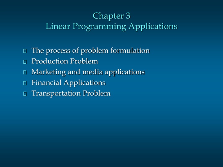
Chapter 3 Linear Programming Applications The process of problem formulation Production Problem Marketing and media applications Financial Applications Transportation Problem
The process of problem formulation Provide a detailed verbal description of the problem Determine the overall objective that appears to be relevant. Determine the factors (constraints) that appear to restrict the attainment of the objective function. Define the decision variables and state their units of measurement. Using these decision variables, formulate an objective function. Formulate a mathematical equations for each of the identified constraints. Check the entire formulation to ensure linearity. 1. 2. 3. 4. 5. 6. 7.
Production Problem The demand for a particular item for a Cosmopolitan Company is known to be: Month January February March Demand 100 110 April 110 120 The production capacity and the cost per unit in these months is, respectively: Month Production Cost ($) January 120 9 February March 150 10 April 100 7 150 8 and the storage cost is $5 per month. At the beginning of January there are 50 items in store, and there should be 80 items left in store at the end of April. Formulate a linear program to find the best production level for each month.
Production Problem Let xibe the amount of production in month i (i=1,2,3,4) Production capacity constraints: x1 120 x2 150 x3 150 x4 100 Amount left over at the end of each month (positive) End of January :50+x1-100 >=0 x1-50 0 End of February: x1-50+x2-110 >=0 x1+x2-160 0 End of March: x1+x2-160+x3-120 >= 0 x1+x2+x3-280 0 End of April: x1+x2+x3-280+x4-110 >= 80 x1+x2+x3+x4-390 80
Production Problem Objective function: Production Cost= 9x1+10x2+8x3+7x4 Storage Cost = 5 [(x1-50)+(x1+x2-160)+(x1+x2+x3- 280)+(x1+x2+x3+x4-390)] Minimize Z = Production Cost + Storage Cost = 29x1+25x2+18x3+13x4-4400 Non-Negativity Constraint : x1, x2, x3, x4 0
Marketing Applications One application of linear programming in marketing is media selection. LP can be used to help marketing managers allocate a fixed budget to various advertising media. The objective is to maximize reach, frequency, and quality of exposure. Restrictions on the allowable allocation usually arise during consideration of company policy, contract requirements, and media availability.
Media Selection SMM Company recently developed a new instant salad machine, has $282,000 to spend on advertising. The product is to be initially test marketed in the Dallas area. The money is to be spent on a TV advertising blitz during one weekend (Friday, Saturday, and Sunday) in November. The three options available are: daytime advertising, evening news advertising, and Sunday game-time advertising. A mixture of one- minute TV spots is desired.
Media Selection Estimated Audience Ad Type Reached With Each Ad Cost Per Ad Daytime 3,000 Evening News 4,000 Sunday Game 75,000 $5,000 $7,000 $100,000 SMM wants to take out at least one ad of each type (daytime, evening-news, and game-time). Further, there are only two game-time ad spots available. There are ten daytime spots and six evening news spots available daily. SMM wants to have at least 5 ads per day, but spend no more than $50,000 on Friday and no more than $75,000 on Saturday.
Media Selection Define the Decision Variables DFR = number of daytime ads on Friday DSA = number of daytime ads on Saturday DSU = number of daytime ads on Sunday EFR = number of evening ads on Friday ESA = number of evening ads on Saturday ESU = number of evening ads on Sunday GSU = number of game-time ads on Sunday
Media Selection Define the Objective Function Maximize the total audience reached: Max (audience reached per ad of each type) x (number of ads used of each type) Max 3000DFR +3000DSA +3000DSU +4000EFR +4000ESA +4000ESU +75000GSU
Media Selection Define the Constraints Take out at least one ad of each type: (1) DFR + DSA + DSU > 1 (2) EFR + ESA + ESU > 1 (3) GSU > 1 Ten daytime spots available: (4) DFR < 10 (5) DSA < 10 (6) DSU < 10 Six evening news spots available: (7) EFR < 6 (8) ESA < 6 (9) ESU < 6
Media Selection Define the Constraints (continued) Only two Sunday game-time ad spots available: (10) GSU < 2 At least 5 ads per day: (11) DFR + EFR > 5 (12) DSA + ESA > 5 (13) DSU + ESU + GSU > 5 Spend no more than $50,000 on Friday: (14) 5000DFR + 7000EFR < 50000
Media Selection Define the Constraints (continued) Spend no more than $75,000 on Saturday: (15) 5000DSA + 7000ESA < 75000 Spend no more than $282,000 in total: (16) 5000DFR + 5000DSA + 5000DSU + 7000EFR + 7000ESA + 7000ESU + 100000GSU7 < 282000 Non-negativity: DFR, DSA, DSU, EFR, ESA, ESU, GSU > 0
Media Selection The Management Scientist Solution Objective Function Value = 199000.000 Variable Value Reduced Costs DFR 8.000 0.000 DSA 5.000 0.000 DSU 2.000 0.000 EFR 0.000 0.000 ESA 0.000 0.000 ESU 1.000 0.000 GSU 2.000 0.000
Media Selection Solution Summary Total new audience reached = 199,000 Number of daytime ads on Friday Number of daytime ads on Saturday = 5 Number of daytime ads on Sunday Number of evening ads on Friday Number of evening ads on Saturday Number of evening ads on Sunday = 1 Number of game-time ads on Sunday = 2 = 8 = 2 = 0 = 0
Financial Planning A bank makes four kinds of loans to its personal customers and these loans yield the following annual interest rates to the bank: First mortgage 14% Second mortgage 20% Home improvement 20% Personal overdraft 10% The bank has a maximum foreseeable lending capability of 250 BD million and is further constrained by the policies: 1. First mortgages must be at least 55% of all mortgages issued and at least 25% of all loans issued (in BD terms) 2. Second mortgages cannot exceed 28% of all loans issued (in BD terms) 3. To avoid public displeasure and the introduction of a new windfall tax the average interest rate on all loans must not exceed 15%. Formulate the bank's loan problem as an LP so as to maximize interest income whilst satisfying the policy limitations.
Financial Planning Define the Decision Variables Essentially we are interested in the amount (in BD) the bank has loaned to customers in each of the four different areas (not in the actual number of such loans). Hence let xi = amount loaned in area i in million of BD (where i=1 corresponds to first mortgages, i=2 to second mortgages i=3 to home improvement, and i=4 to personal overdraft)
Financial Planning Define the Objective Function To maximize interest income (which is given above) Maximize Z=0.14x1 + 0.20x2 + 0.20x3 + 0.10x4 Define the Constraints (a) Limit on amount lent x1 + x2 + x3 + x4 250 (b) Policy condition 1 x1 0.55(x1 + x2) i.e. first mortgages >= 0.55(total mortgage lending) and also x1 0.25(x1 + x2 + x3 + x4) i.e. first mortgages >= 0.25(total loans)
Financial Planning Define the Constraints (continued) c) policy condition 2 x2 0.28(x1 + x2 + x3 + x4) d) policy condition 3 we know that the total annual interest is 0.14x1 + 0.20x2 + 0.20x3 + 0.10x4 on total loans of (x1 + x2 + x3 + x4). Hence the constraint relating to policy condition (3) is: 0.14x1 + 0.20x2 + 0.20x3 + 0.10x4 0.15(x1 + x2 + x3 + x4) Non-Negativity Constraint: xi 0 (i=1,2,3,4)
Transportation Problem The transportation problem seeks to minimize the total shipping costs of transporting goods from m origins (each with a supply si) to n destinations (each with a demand dj), when the unit shipping cost from an origin, i, to a destination, j, is cij. The network representation for a transportation problem with two sources and three destinations is given on the next slide.
Transportation Problem Network Representation d1 1 c11 c12 1 s1 c13 c21 d2 2 c22 s2 2 c23 d3 3 Sources Destinations
Transportation Problem Steel Mills in three cities produce the following amounts of steel: Location Production (tons) A 150 B C 210 320 These mills supply steel to four cities, where manufacturing plants have the following demands: Plants 1 Demand (tons) 190 2 3 4 70 180 240 The cost of sending 1 tons of steel from a production location to a plant depends on the distance the truck must travel. The problem is to determine how many tons of steel to transport from each production mill to each manufacturing plant on a weekly basis to minimize the total cost of transportation. Formulate the above problem as a linear programming model.
Transportation tableau A transportation problem is specified by the supply, the demand, and the shipping costs. So the relevant data can be summarized in a transportation tableau. The transportation tableau implicitly expresses the supply and demand constraints and the shipping cost between each demand and supply point. From To Plant 3 $16 $7 $10 180 1 2 4 Supply (tons) 150 210 320 A B C $14 $11 $16 190 $9 $8 $12 70 $18 $16 $22 240 Demand (tons) 23
Transportation Problem Decision Variable: Let Xij = number of tons of steel shipped from location i to plant j (i = A, B, C; j = 1, 2, 3, 4) Objective function Transportation costs of steel shipped from location A = 14 XA1 + 9 XA2 +16 XA3 +18 XA4 Transportation costs of steel shipped from location B = 11 XB1 + 8 XB2 + 7 XB3 +16 XB4 Transportation costs of steel shipped from location C = 16 XC1 + 12 XC2+ 10 XC3+22 XC4 Therefore, the objective function is: Minimize 14 XA1+ 9 XA2+16 XA3+18 XA4+ 11 XB1+ 8 XB2+ 7 XB3 +16 XB4+ 16 XC1+ 12 XC2+ 10 XC3+22 XC4 24
Transportation Problem 3. Supply Constraints Since each supply point has a limited production capacity; XA1 + XA2 + XA3 + XA4 150 XB1 + XB2 + XB3 + XB4 210 XC1+ XC2+ XC3+ XC4 320 25
Transportation Problem 4. Demand Constraints Since each supply point has a limited production capacity; XA1+ XB1+ XC1 190 XA2 + XB2+ XC2 70 XA3+ XB3+ XC3 180 XA4 + XB4 + XC4 240 5. Sign Constraints Xij 0 (i= A,B,C; j= 1,2,3,4) 26
