Linear Programming Application in Marketing: Media Selection for SMM Company
SMM Company, a salad machine manufacturer, aims to optimize its advertising budget of $282,000 for a new product launch in Dallas. By utilizing linear programming, the company seeks to maximize audience reach through TV ads while adhering to specific constraints such as ad types, budget limitations, and available ad spots.
Download Presentation

Please find below an Image/Link to download the presentation.
The content on the website is provided AS IS for your information and personal use only. It may not be sold, licensed, or shared on other websites without obtaining consent from the author.If you encounter any issues during the download, it is possible that the publisher has removed the file from their server.
You are allowed to download the files provided on this website for personal or commercial use, subject to the condition that they are used lawfully. All files are the property of their respective owners.
The content on the website is provided AS IS for your information and personal use only. It may not be sold, licensed, or shared on other websites without obtaining consent from the author.
E N D
Presentation Transcript
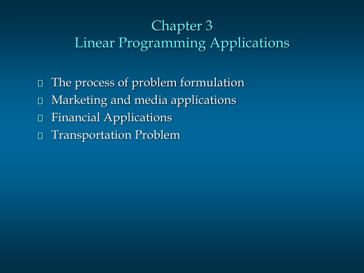
Chapter 3 Linear Programming Applications The process of problem formulation Marketing and media applications Financial Applications Transportation Problem
The process of problem formulation Provide a detailed verbal description of the problem Determine the overall objective that appears to be relevant. Determine the factors (constraints) that appear to restrict the attainment of the objective function. Define the decision variables and state their units of measurement. Using these decision variables, formulate an objective function. Formulate a mathematical equations for each of the identified constraints. Check the entire formulation to ensure linearity. 1. 2. 3. 4. 5. 6. 7.
Marketing Applications One application of linear programming in marketing is media selection. LP can be used to help marketing managers allocate a fixed budget to various advertising media. The objective is to maximize reach, frequency, and quality of exposure. Restrictions on the allowable allocation usually arise during consideration of company policy, contract requirements, and media availability.
Media Selection SMM Company recently developed a new instant salad machine, has $282,000 to spend on advertising. The product is to be initially test marketed in the Dallas area. The money is to be spent on a TV advertising blitz during one weekend (Friday, Saturday, and Sunday) in November. The three options available are: daytime advertising, evening news advertising, and Sunday game-time advertising. A mixture of one- minute TV spots is desired.
Media Selection Estimated Audience Ad Type Reached With Each Ad Cost Per Ad Daytime 3,000 Evening News 4,000 Sunday Game 75,000 $5,000 $7,000 $100,000 SMM wants to take out at least one ad of each type (daytime, evening-news, and game-time). Further, there are only two game-time ad spots available. There are ten daytime spots and six evening news spots available daily. SMM wants to have at least 5 ads per day, but spend no more than $50,000 on Friday and no more than $75,000 on Saturday.
Media Selection Define the Decision Variables DFR = number of daytime ads on Friday DSA = number of daytime ads on Saturday DSU = number of daytime ads on Sunday EFR = number of evening ads on Friday ESA = number of evening ads on Saturday ESU = number of evening ads on Sunday GSU = number of game-time ads on Sunday
Media Selection Define the Objective Function Maximize the total audience reached: Max (audience reached per ad of each type) x (number of ads used of each type) Max 3000DFR +3000DSA +3000DSU +4000EFR +4000ESA +4000ESU +75000GSU
Media Selection Define the Constraints Take out at least one ad of each type: (1) DFR + DSA + DSU > 1 (2) EFR + ESA + ESU > 1 (3) GSU > 1 Ten daytime spots available: (4) DFR < 10 (5) DSA < 10 (6) DSU < 10 Six evening news spots available: (7) EFR < 6 (8) ESA < 6 (9) ESU < 6
Media Selection Define the Constraints (continued) Only two Sunday game-time ad spots available: (10) GSU < 2 At least 5 ads per day: (11) DFR + EFR > 5 (12) DSA + ESA > 5 (13) DSU + ESU + GSU > 5 Spend no more than $50,000 on Friday: (14) 5000DFR + 7000EFR < 50000
Media Selection Define the Constraints (continued) Spend no more than $75,000 on Saturday: (15) 5000DSA + 7000ESA < 75000 Spend no more than $282,000 in total: (16) 5000DFR + 5000DSA + 5000DSU + 7000EFR + 7000ESA + 7000ESU + 100000GSU7 < 282000 Non-negativity: DFR, DSA, DSU, EFR, ESA, ESU, GSU > 0
Media Selection The Management Scientist Solution Objective Function Value = 199000.000 Variable Value Reduced Costs DFR 8.000 0.000 DSA 5.000 0.000 DSU 2.000 0.000 EFR 0.000 0.000 ESA 0.000 0.000 ESU 1.000 0.000 GSU 2.000 0.000
Media Selection Solution Summary Total new audience reached = 199,000 Number of daytime ads on Friday Number of daytime ads on Saturday = 5 Number of daytime ads on Sunday Number of evening ads on Friday Number of evening ads on Saturday Number of evening ads on Sunday = 1 Number of game-time ads on Sunday = 2 = 8 = 2 = 0 = 0
Financial Applications LP can be used in financial decision-making that involves capital budgeting, make-or-buy, asset allocation, portfolio selection, financial planning, and more. Portfolio selection problems involve choosing specific investments for example, stocks and bonds from a variety of investment alternatives. This type of problem is faced by managers of banks, mutual funds, and insurance companies. The objective function usually is maximization of expected return or minimization of risk.
Portfolio Selection Winslow Savings has $20 million available for investment. It wishes to invest over the next four months in such a way that it will maximize the total interest earned over the four month period as well as have at least $10 million available at the start of the fifth month for a high rise building venture in which it will be participating.
Portfolio Selection For the time being, Winslow wishes to invest only in 2-month government bonds (earning 2% over the 2-month period) and 3-month construction loans (earning 6% over the 3-month period). Each of these is available each month for investment. Funds not invested in these two investments are liquid and earn 3/4 of 1% per month when invested locally.
Portfolio Selection Formulate a linear program that will help Winslow Savings determine how to invest over the next four months if at no time does it wish to have more than $8 million in either government bonds or construction loans.
Portfolio Selection Define the Decision Variables Gi = amount of new investment in government bonds in month i (for i = 1, 2, 3, 4) Ci = amount of new investment in construction loans in month i (for i = 1, 2, 3, 4) Li = amount invested locally in month i, (for i = 1, 2, 3, 4)
Portfolio Selection Define the Objective Function Maximize total interest earned in the 4-month period: Max (interest rate on investment) X (amount invested) Max .02G1 + .02G2 + .02G3 + .02G4 + .06C1 + .06C2 + .06C3 + .06C4 + .0075L1 + .0075L2 + .0075L3 + .0075L4
Portfolio Selection Define the Constraints Month 1's total investment limited to $20 million: (1) G1 + C1 + L1 = 20,000,000 Month 2's total investment limited to principle and interest invested locally in Month 1: (2) G2 + C2 + L2 = 1.0075L1 or G2 + C2 - 1.0075L1 + L2 = 0
Portfolio Selection Define the Constraints (continued) Month 3's total investment amount limited to principle and interest invested in government bonds in Month 1 and locally invested in Month 2: (3) G3 + C3 + L3 = 1.02G1 + 1.0075L2 or - 1.02G1 + G3 + C3 - 1.0075L2 + L3 = 0
Portfolio Selection Define the Constraints (continued) Month 4's total investment limited to principle and interest invested in construction loans in Month 1, goverment bonds in Month 2, and locally invested in Month 3: (4) G4 + C4 + L4 = 1.06C1 + 1.02G2 + 1.0075L3 or - 1.02G2 + G4 - 1.06C1 + C4 - 1.0075L3 + L4 = 0 $10 million must be available at start of Month 5: (5) 1.06C2 + 1.02G3 + 1.0075L4 > 10,000,000
Portfolio Selection Define the Constraints (continued) No more than $8 million in government bonds at any time: (6) G1 < 8,000,000 (7) G1 + G2 < 8,000,000 (8) G2 + G3 < 8,000,000 (9) G3 + G4 < 8,000,000
Portfolio Selection Define the Constraints (continued) No more than $8 million in construction loans at any time: (10) C1 (11) C1 + C2 (12) C1 + C2 + C3 (13) C2 + C3 + C4 < 8,000,000 < 8,000,000 < 8,000,000 < 8,000,000 Non-negativity: Gi, Ci, Li > 0 for i = 1, 2, 3, 4
Portfolio Selection The Management Scientist Solution Objective Function Value = 1429213.7987 Variable Value Reduced Costs G1 8000000.0000 0.0000 G2 0.0000 0.0000 G3 5108613.9228 0.0000 G4 2891386.0772 0.0000 C1 8000000.0000 0.0000 C2 0.0000 0.0453 C3 0.0000 0.0076 C4 8000000.0000 0.0000 L1 4000000.0000 0.0000 L2 4030000.0000 0.0000 L3 7111611.0772 0.0000 L4 4753562.0831 0.0000
Transportation Problem The transportation problem seeks to minimize the total shipping costs of transporting goods from m origins (each with a supply si) to n destinations (each with a demand dj), when the unit shipping cost from an origin, i, to a destination, j, is cij. The network representation for a transportation problem with two sources and three destinations is given on the next slide.
Transportation Problem Network Representation d1 1 c11 c12 1 s1 c13 c21 d2 2 c22 s2 2 c23 d3 3 Sources Destinations
Transportation Problem LP Formulation The LP formulation in terms of the amounts shipped from the origins to the destinations, xij , can be written as: i j s.t. xij < si for each origin i j xij djfor each destination j i xij > 0 for all i and j Min cijxij
Transportation Problem Powerco has three electric power plants that supply the electric needs of four cities. The associated supply of each plant and demand of each city is given in the table 1. The cost of sending 1 million kwh of electricity from a plant to a city depends on the distance the electricity must travel. A transportation problem is specified by the supply, the demand, and the shipping costs. So the relevant data can be summarized in a transportation tableau. The transportation tableau implicitly expresses the supply and demand constraints and the shipping cost between each demand and supply point.
Transportation tableau From To City 1 City 2 City 3 City 4 Supply (Million kwh) 35 50 40 Plant 1 Plant 2 Plant 3 Demand (Million kwh) $8 $9 $14 45 $6 $12 $9 20 $10 $13 $16 30 $9 $7 $5 30 Transportation Tableau 29
Transportation Problem Decision Variable: Since we have to determine how much electricity is sent from each plant to each city; Xij = Amount of electricity produced at plant i and sent to city j X14 = Amount of electricity produced at plant 1 and sent to city 4 1. 30
Transportation Problem 2. Objective function Since we want to minimize the total cost of shipping from plants to cities; Minimize Z = 8X11+6X12+10X13+9X14 +9X21+12X22+13X23+7X24 +14X31+9X32+16X33+5X34 31
Transportation Problem 3. Supply Constraints Since each supply point has a limited production capacity; X11+X12+X13+X14 <= 35 X21+X22+X23+X24 <= 50 X31+X32+X33+X34 <= 40 32
Transportation Problem 4. Demand Constraints Since each supply point has a limited production capacity; X11+X21+X31 >= 45 X12+X22+X32 >= 20 X13+X23+X33 >= 30 X14+X24+X34 >= 30 33
Transportation Problem 5. Sign Constraints Since a negative amount of electricity can not be shipped all Xij s must be non negative; Xij >= 0 (i= 1,2,3; j= 1,2,3,4) 34
LP Formulation of Powercos Problem Min Z = 8X11+6X12+10X13+9X14+9X21+12X22+13X23+7X24 +14X31+9X32+16X33+5X34 S.T.: X11+X12+X13+X14 <= 35 X21+X22+X23+X24 <= 50 X31+X32+X33+X34 <= 40 X11+X21+X31 >= 45 X12+X22+X32 >= 20 X13+X23+X33 >= 30 X14+X24+X34 >= 30 Xij >= 0 (i= 1,2,3; j= 1,2,3,4) (Supply Constraints) (Demand Constraints) 35
