Learning Bayesian Network Models from Complex Relational Data

Delve into the process of learning Bayesian network models from complex relational data, extending traditional algorithms to suit relational data structures. Explore key concepts like likelihood functions, graphical model initialization, and parameter learning for effective model fitting.

• Bayesian Networks
• Relational Data
• Graphical Models
• Parameter Learning
• Likelihood Functions

shey764 Follow

Uploaded on Nov 24, 2024 | 0 Views

Download Presentation

Please find below an Image/Link to download the presentation.

The content on the website is provided AS IS for your information and personal use only. It may not be sold, licensed, or shared on other websites without obtaining consent from the author. Download presentation by click this link. If you encounter any issues during the download, it is possible that the publisher has removed the file from their server.

Presentation Transcript

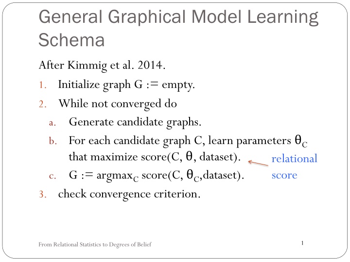
1. General Graphical Model Learning Schema After Kimmig et al. 2014. 1. Initialize graph G := empty. 2. While not converged do a. Generate candidate graphs. b. For each candidate graph C, learn parameters C that maximize score(C, , dataset). c. G := argmaxCscore(C, C,dataset). 3. check convergence criterion. relational score 1 From Relational Statistics to Degrees of Belief

2. Parameter Learning Section 3 Tutorial on Learning Bayesian Networks for Complex Relational Data

3. Overview: Upgrading Parameter Learning Extend learning concepts/algorithms designed for iid data to relational data This is called upgrading iid learning (van de Laer and De Raedt) Score/Objective Function: Random Selection Likelihood Algorithm: Fast M bius Transform van de Laer, W. & De Raedt, L. (2001), How to upgrade propositional learners to first-order logic: A case study , in Relational Data Mining', Springer Verlag 3

4. Likelihood Function for IID Data Learning Bayesian Networks for Complex Relational Data

5. Score-based Learning for IID data Most Bayesian network learning methods are based on a score function The score function measures how well the network fits the observed data Key component: the likelihood function. measures how likely each datapoint is according to the Bayesian network data table Bayesian Network Log-likelihood, e.g. -3.5 5 Learning Bayesian Networks for Complex Relational Data

6. The Bayes Net Likelihood Function for IID data 1. For each row, compute the log-likelihood for the attribute values in the row. 2. Log-likelihood for table = sum of log-likelihoods for rows. 6

7. IID Example P(Action(M.)=T) = 1 Action(Movie) Drama(Movie) Title Fargo Kill_Bill Drama Action Horror T T F T F F P(Drama(M.)=T|Action(M.)=T) = 1/2 Horror(Movie) P(Horror(M.)=F|...) = 1 Title Fargo Kill_Bill Drama Action HorrorPB F F ln(PB) T F T T 1x1/2x1 = 1/2 1x1/2x1 = 1/2 -0.69 -0.69 Total Log-likelihood Score for Table = -1.38 7 Learning Bayesian Networks for Complex Relational Data

8. Likelihood Function for Relational Data Learning Bayesian Networks for Complex Relational Data

9. Wanted: a likelihood score for relational data database Problems Multiple Tables. Dependent data points Bayesian Network Log-Likelihood, e.g. -3.5 9 Learning Bayesian Networks for Complex Relational Data

10. The Random Selection Likelihood Score 1. Randomly select a grounding/instantiation for all first-order variables in the first-order Bayesian network 2. Compute the log-likelihood for the attributes of the selected grounding 3. Log-likelihood score = expected log-likelihood for a random grounding Generalizes IID log-likelihood, but without independence assumption Schulte, O. (2011), A tractable pseudo-likelihood function for Bayes Nets applied to relational data, in 'SIAM SDM', pp. 462-473. 10

11. Example P(g(A)=M) = 1/2 gender(A) P(ActsIn(A,M)=T|g(A)=M) = 1/4 P(ActsIn(A,M)=T|g(A)=W) = 2/4 ActsIn(A,M) Pro b A M gender(A ) M M W W M M W W ActsIn(A,M) PB ln(PB) F F F T T F F T 3/8 3/8 2/8 2/8 1/8 3/8 2/8 2/8 0.27 geo-1.32 arith 1/8 1/8 1/8 1/8 1/8 1/8 1/8 1/8 Brad_Pitt Brad_Pitt Lucy_Liu Lucy_Liu Steve_Buscemi Fargo Steve_Buscemi Kill_Bill Uma_ThurmanFargo Uma_ThurmanKill_Bill Fargo Kill_Bill Fargo Kill_Bill -0.98 -0.98 -1.39 -1.39 -2.08 -0.98 -1.39 -1.39 11

12. Observed Frequencies Maximize Random Selection Likelihood Proposition The random selection log-likelihood score is maximized by setting the Bayesian network parameters to the observed conditional frequencies gender(A) P(g(A)=M) = 1/2 P(ActsIn(A,M)=T|g(A)=M) = 1/4 P(ActsIn(A,M)=T|g(A)=W) = 2/4 ActsIn(A,M) Schulte, O. (2011), A tractable pseudo-likelihood function for Bayes Nets applied to relational data, in 'SIAM SDM', pp. 462-473. 12

13. Computing Maximum Likelihood Parameter Values The Parameter Values that maximize the Random Selection Likelihood Learning Bayesian Networks for Complex Relational Data

14. Computing Relational Frequencies Need to compute a contingency table with instantiation counts Well researched for all true relationships SQL Count(*) Virtual Join Partition Function Reduction g(A) Acts(A,M) M M W W M M W W action(M) count 3 3 2 2 1 3 2 2 F F F T T F F T T T T T T T T T Yin, X.; Han, J.; Yang, J. & Yu, P. S. (2004), CrossMine: Efficient Classification Across Multiple Database Relations, in 'ICDE'. Venugopal, D.; Sarkhel, S. & Gogate, V. (2015), Just Count the Satisfied Groundings: Scalable Local- Search and Sampling Based Inference in MLNs, in AAAI, 2015, pp. 3606--3612. 14

15. Single Relation Case For single relation compute PD (R = F) using 1-minus trick (Getoor et al. 2003) Example: PD(HasRated(User,Movie) = T) = 4.27% PD(HasRated(User,Movie) = F) = 95.73% How to generalize to multiple relations? PD(ActsIn(Actor,Movie)=F,HasRated(User,Movie)=F) Getoor, L.; Friedman, N.; Koller, D. & Taskar, B. (2003), 'Learning probabilistic models of link structure', J. Mach. Learn. Res. 3, 679--707. 15

16. The Mbius Extension Theorem for negated relations For two link types R1 R1 R1 R2 R2 R2 p4 p3 p2 Joint probabilities R1 R2 p1 R1 R1 R2 q4 q3 q2 q1 M bius Parameters R2 nothing 16 Learning Bayesian Networks for Complex Relational Data

17. The Fast Inverse Mbius Transform ActsIn(A,M) = R1 HasRated(U,M) = R2 Initial table with no false relationships Table with joint probabilities J.P. = joint probability R1 T * T * R2 J.P. T T * * R1 T F T F R2 J.P. T T * * R1 T F T F R2 J.P. T T F F 0.2 0.3 0.4 1 0.2 0.1 0.4 0.6 0.2 0.1 0.2 0.5 - + - + - - + + Kennes, R. & Smets, P. (1990), Computational aspects of the M bius transformation, in 'UAI', pp. 401-416. 17

18. Parameter Learning Time Fast Inverse M bius transform (IMT) vs Constructing complement tables using SQL Times are in seconds M bius transform is much faster, 15-200 times 18 Learning Bayesian Networks for Complex Relational Data

19. Using Presence and Absence of Relationships Find correlations between links/relationships, not just attributes given links If a user performs a web search for an item, is it likely that the user watches a movie about the item? Example of Weka-interesting association rule on Financial benchmark dataset: statement_frequency(Account) = monthly HasLoan(Account, Loan) = true Qian, Z.; Schulte, O. & Sun, Y. (2014), Computing Multi-Relational Sufficient Statistics for Large Databases, in 'Computational Intelligence and Knowledge Management (CIKM)', pp. 1249--1258. 19

20. Summary Random Selection Semantics random selection log-likelihood Maximizing values for random selection log-likelihood = observed empirical frequencies. Generalizes maximum likelihood result for IID data. Fast M bius Transform: computes database frequencies for conjunctive formulas involving any number of negative relationships. Enables link analysis: modelling probabilistic associations that involve the presence or absence of relationships. 20 Learning Bayesian Networks for Complex Relational Data