Laplace Transforms: Understanding Analysis and Examples
Explore the concepts of Laplace Transforms, structural identifiability analysis, and key examples taught at the University of Warwick's AMR Summer School by Dr. Mike Chappell. Delve into the mathematics behind Laplace Transforms and learn how to find the transform of different functions, including constants and exponential functions. Gain insights into the inverse Laplace Transform pairs and common transform pairs for a deeper understanding of this integral transform technique.

Download Presentation

Please find below an Image/Link to download the presentation.
The content on the website is provided AS IS for your information and personal use only. It may not be sold, licensed, or shared on other websites without obtaining consent from the author. If you encounter any issues during the download, it is possible that the publisher has removed the file from their server.
You are allowed to download the files provided on this website for personal or commercial use, subject to the condition that they are used lawfully. All files are the property of their respective owners.
The content on the website is provided AS IS for your information and personal use only. It may not be sold, licensed, or shared on other websites without obtaining consent from the author.
E N D
Presentation Transcript
University of Warwick: AMR Summer School 4th-6thJuly, 2016 Structural Identifiability Analysis Dr Mike Chappell, School of Engineering, University of Warwick. Laplace Transforms DR. MIKE CHAPPELL OFFICE: D216 - Email: M.J.Chappell@warwick.ac.uk
Pierre-Simon LAPLACE 1749-1827 2
LAPLACE TRANSFORMS For a piecewise continuous function f (t), t 0 the Laplace Transform is defined as: L = st ( ) ( ) f t ( ) s e f t dt (*) 0 = Often denoted by L ( ) ( ) f t F s ( ) f t t s F s An integral transform: transforms ( ) Note: The transform only exists when the improper integral (*) exists (i.e. is finite) LAPLACE TRANSFORM 3
Examples = ( ) f t k (1) What is the Laplace transform of ( k constant, t 0) k = = st ( ) L F s e kdt By definition: 0 k e dt = st 0 1 s = st k e 0 k s = (Note: exists for s>0) LAPLACE TRANSFORM - EXAMPLE 4
Examples = at ( ) f t e (2) What is the Laplace transform of (t 0) e = By definition: = at st at ( ) L F s e e dt 0 = a s t ( ) e dt 0 1 a s t = ( ) e ( ) a s 0 1 = (Note: exists for s>a) s a Only a function of s LAPLACE TRANSFORM - EXAMPLE 5
Laplace Transform pairs If then by taking inverses we can, knowing F(s), ( ) ( ) f t F s = L ( ) (s) f t F = L 1 L L 1 obtain f (t) and give a Laplace Transform pair Both satisfy linearity conditions: L + = = = = + L ( ) L ( ) L k ( ) f t F s L L ( ) f t g t . ( ) k f t + . ( ) F s f t g t . ( ) ( k constant) For inverses: 1 1 1 + L ( ) ( ) L ( ) F s L ( ) F s L G s G s 1 1 . ( ) ( constant) The Laplace transform pairs for the most common cases are given in Tables (in the textbook and more importantly in your Data Books) LAPLACE TRANSFORM PAIRS 6
Examples: Find the Laplace Transforms of: (1) Note: ( ) 5 f t e = e 2 t = 2 2 t t L 5 1 5 L e e Tables give Laplace transform of eat : 5 e L = at L s a 1 So a=2 = 2 t 5 2 s 5 = 2 s = ( ) sin3 f t t (2) + = L sin t Tables give Laplace transformsin t: 2 2 s 3 + Here =3 = L sin3 t 2 9 s LAPLACE TRANSFROM - EXAMPLE 8
Examples: (3) From Tables: ( ) cos3 f t e = + s a a + = 5 t at t L cos e t + 2 2 ( ) s + 5 s So a=5, =3 = 5 t L cos3 e t + + 2 ( 5) 9 s 1 2 = + 2 t ( ) e 3sin4 f t t (4) 1 2 1 2 + = + 2 2 t t L e 3sin4 L e 3 L sin4 t t By linearity: 1 2 1 2 ( 1 2 ( 1 + 1 + 4 + + = + Solving from Tables: 2 t L e 3 L sin4 3 t 2 2) ( 16) s s 12 + = + 2 2) ( 16) s s LAPLACE TRANSFORM - EXAMPLE 9
Examples: Find the Inverse Laplace transforms of: 1 ( ) 5 s 1 5 s 1 e = at (1) from Tables: F s = L s a So a=5 = 1 5 t L e 5 ! + N s t = (2) from Tables: 3 ( ) F s s = N L 1 N 5 2t 5 s 5 2 2 s So N=2 1 1 = = 2 L L 3 3 INVERSE LAPLACE TRANSFORM - EXAMPLE 10
Examples: 4 3 + 4 s = + (3) 4 ( ) F s s 2 4 s 3 + 4 s 3 + By Linearity 1 1 1 + = + L L L 4 2 4 2 4 4 s s 2 3t ! + N s 4 s 4 6 6 s t = 3 = 1 1 = N L L L from Tables: 4 4 1 N + 3 + 3 2 2 + 3sin2 2 1 1 = = = L sin t L L t 2 2 2 2 4 4 s s s 4 s 3 + 2 3 3sin2 2 + = + 1 3 L t t Hence 4 2 4 s INVERSE LAPLACE TRANSFORM - EXAMPLE 11
Note: You may need to use partial fractions; i.e. find 4 1 L + 2 ( 1)( 1) s s + + 4 A Bs C s = + By partial fractions: + 2 2 ( 1)( = 1) + ( 1) + ( 1) s s s 1) ( + 2 4 ( )( 1) A s Bs C s = = + = = 2: 0 : 0 Let compare coeffs. 1 2 s A = = 2 2 s s A C B B B C 4 1 1 s + 1 1 1 1 = L 2 L 2 L 2 L So + + 2 2 2 ( 1)( 1) ( 1) ( 1) ( 1) s s s s s = te 2 2cos t 2sin t From tables: INVERSE LAPLACE TRANSFORM - EXAMPLE 12
Note: You may also need to use completing the square 3 2 1 i.e. find 2 s L + + (Denominator will not factorise) 5 s = 3 2 3 1 Completing square gives: 1 L L + + + + 2 2 5 ( 1) 4 s s s 3 2 2 = 1 L + + 2 ( 1) 4 s 3 2 = From tables: t sin2 e t INVERSE LAPLACE TRANSFORM - EXAMPLE 13
Laplace Transform of Derivatives dyt dt = Consider y(t) such that , what is ? L ( ) L ( ) y t ( ) Y s dyt dt stdy dt = L ( ) ( ) t dt e By definition 0 dv dt dy dt du dt = = = = st st ; ; Use parts u e se v y dyt dt s e So = + st st L ( ) ( ) y t e ( ) y t dt 0 0 = + (0) ( ) y sY s dy dt (0) = 2 d yt dt = dyt 2 L 2( ) ( ) (0) '(0) So , similarly ( ) ( ) sY s dt s Y s sy y L (0) y LAPLACE TRANSFORM OF DERIVATIVES 14
Example: 2 d y dy = = If find given 2 " ; ' y y dt dt " 2 ' 5 " y y y y + = L L 2( ) s Y s = s Y s = ( 2 s s = + " 2 ' 5 y + (0) 1 ; '(0) = = L 3 y y y y y (0) 3 2( 5) ( ) Y s y ( ) 1) 5 ( ) sY s 1 s + y 2 sy s L ' 5 L (0)) 5 ( ) + '(0) 2( ( ) + sY s y Y s 2( ) Y s 2 (*) Note: DIFFERENTIAL EQUATION BECOMES ALGEBRAIC If . Take Laplace transforms, then (*) gives: " 2 ' 5 0 y y y + = 1 ( ) 2 5 s s + + s 1 2 s = = + Y s + + 2 2 2 ( 1) 4 ( 1) 4 s s and taking the inverse Laplace transform to give y(t) yields: ( ) cos2 y t e = + t t sin2 t e t No arbitrary constants, Immediate solution including i.c .s LAPLACE TRANSFORM OF DERIVATIVES - EXAMPLE 15
Solution for initial value problems Solving linear ODEs with given initial conditions algebraically Examples: d y dt 2 + = = = (1) cos , (0) t 0 , '(0) 1 y y y 2 Take Laplace transforms on both sides of the equation: " y + = L L cos y t s + + = 2 ( ) (0) '(0) ( ) s Y s sy y Y s 2 1 s s + + = 2 ( 1) ( ) Y s .0 1 s s 2 1 s 1 s + = + ( ) Y s Rearranging gives: + 2 2 2 ( 1) ( 1) ( ) y t s s 1 2 1( 2 = + = + sin sin 1)sin t t t t t Taking inverse Laplace transforms gives: SOLUTION OF INITIAL VALUE PROBLEMS 16
Examples: " 3 ' 2 y + + = , (0) 1 , '(0) 1 y = = t y y e y (2) Take Laplace transforms on both sides of the equation: 1 '(0) 3( + (0)) 2 ( ) + = 2 ( ) (0) ( ) s Y s sy y sY s y Y s 1 s 1 4 s 1 + + = + + = + + 2 2 ( 3 2) ( ) Y s 1 3 ( 3 2) ( ) Y s 4 s s s s s s 1 1 s s + 1 s + = + ( ) Y s + s + s + + 2 2 ( 1)( s 3 2) ( 3 2) s s s s + 2 3 3 s 3 s = + 2 ( 1)( s 3 2) s s + 2 3 + = 2) Using partial fractions + ( 1)( 1)( s s SOLUTION OF INITIAL VALUE PROBLEMS 17
Examples: " 3' 2 + + = , (0) 1 , '(0) 1 y = = t y y e y (2) (cont) + 2 3 + 3 s s s A B + C + = + + Using partial fractions: + ( 1)( 1)( 2) ( 1) ( 1) ( 2) s s s s s + = + + + + + + 2 3 3 ( 1)( 2) ( 1)( 2) ( 1)( 1) s s A s s B s s C s s i.e. 1 6 = = = 1 1 6 A s A So 1 6 ( 1 5 2 ( 1 + 5 3 ( 1 + 5 2 5 3 = = = 1 5 2 B s B = + ( ) Y s 1) 1) 2) s s s = = = 2 5 3 C s C 1 6 5 2 5 3 Taking inverse Laplace transforms gives: = + 2 t t t ( ) y t e e e SOLUTION OF INITIAL VALUE PROBLEMS 18
INTRODUCTION TO SYSTEMS THEORY 2 d x dx dt Consider system equation (1) 2 a dt + + = ( ) bx u t = with observation/measurement (2) ( ) y t ( ) cx t Assume all initial conditions are zero (i.e. y(0)=y (0)=0) Take Laplace Transforms of (1) and (2) to give: ( ) ( ) X s s as b + + (3) (4) + + = = 2 ( ) ( ) ( ) ( ) ( ) ( ) s X s asX s Y s bX s cX s U s U s = From (3) 2 c as b + = Substitute for X(s) in (4) to give: = ( ) ( ) Y s U s The Transfer Function (relates input to output) + 2 s ( ) ( ) Y s U s c as b + = OR ( ) G s + 2 s INTRODUTION TO SYSTEMS THEORY 19
In block diagram form ( ) ( ) U s Y s c as b + = ( ) G s + 2 s Set to give the Fourier transform ( 1) s i i = = c = ( ) G i + 2 ( ) b ia INTRODUTION TO SYSTEMS THEORY OF FREQUENCY RESPONSE IN ES18 20