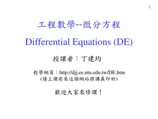
Solving LTI ODE Using Laplace and Fourier Transforms
Laplace transform
Define auxiliary function
g
(
,
t
):
Pb. 1:
if lim
t
f
(
t
)
0:
FT is not defined
Pb. 2:
FT does
not
capture well sinusoidal with damping/divergence
Fourier transform (FT) has 2 problems:
Its FT is:
Laplace transform:
Inverse Laplace
Laplace transform properties
Independent
variable:
t
Dependent
variable:
y
Function is a
mapping:
y
=
f
(
t
)
Time domain
t
y
f
(
t
)
F
(
s
)
e
–
at
1/(
s+a
)
sin(
at
)
a
/(
s
2
+a
2
)
cos(
at
)
s
/(
s
2
+a
2
)
(
t
)
1 /
s
t
k
/k!
(
k
0)
1
/
s
k+
1
f
(
t
)
F
(
s
)
g
(
t
)=
df
(
t
)/
dt
G
(
s
)
=s F
(
s
) –
f
(0)
g
(
t
)=
f
(
t
)
dt
G
(
s
)
=
(1/
s
)
F
(
s
)
g
(
t
)=
(
t–a
)
f
(
t–a
)
G
(
s
)
=
(e
–
at
)
F
(
s
)
g
(
t
) = e
–
at
f
(
t
)
G
(
s
)
=F
(
s+a
)
Application to solve LTI – ODE
Take
: m
=2,
c
=4,
k
=20, and
f
1
=60
Inverse transform
To get the inverse transform: Partial fractions
Required to inverse:
1.
Get factors
of
D
n
(
s
):
First get solutions of D
n
(
s
)
=
0: say
p
1
,
p
2
, …,
p
n
D
n
(
s
) = (
s
–
p
1
) (
s
–
p
2
) … (
s
–
p
n
)
2.
If complex
conjugate solutions:
p
1
=
+
j
,
p
2
=
–
j
,
group: (
s
–
p
1
) (
s
–
p
2
)
= (
s
2
+ 2
s
+
2
+
2
)
= ((
s
+
)
2
+
2
)
G
(
s
) =
N
m
(
s
) /
D
n
(
s
)
3.
Rewrite
G
(
s
) as:
4.
Get
A
i
by recombining the RHS
and comparing with LHS
N
&
D
are polynomials in
s
of degree
m
,
n
:
n
m
f
(
t
)
F
(
s
)
(
t
)
1 /
s
t
k
/k!
(
k
0)
1
/
s
k+
1
e
–
at
1/(
s+a
)
e
–
bt
f
(
t
)
F
(
s+b
)
sin(
at
)
a
/(
s
2
+a
2
)
cos(
at
)
s
/(
s
2
+a
2
)
Get the inverse from:
To get the inverse transform:
To get the inverse of:
1. Get factors of the denominator:
s
(
s+a
) (
s+b
)
[where:
a
= – 1 + 3
j
,
b
= – 1 – 3
j
]; [Note that (
s+a
)(
s+b
) = (
s
+1)
2
+ 3
2
]
2. Expand original fraction to partial fractions:
Use partial fractions
3. Get numerators by equating both sides
4. Use tables
f
(
t
)
F
(
s
)
(
t
)
1 /
s
t
k
/k!
(
k
0)
1
/
s
k+
1
e
–
at
1/(
s+a
)
e
–
bt
f
(
t
)
F
(
s+b
)
sin(
at
)
a
/(
s
2
+a
2
)
cos(
at
)
s
/(
s
2
+a
2
)
Application of Laplace and Fourier transforms to solve Linear Time-Invariant Ordinary Differential Equations (LTI ODEs) with specific functions and parameters. Learn how to find the inverse transform using partial fractions and handle complex solutions.

Download Presentation

Please find below an Image/Link to download the presentation.
The content on the website is provided AS IS for your information and personal use only. It may not be sold, licensed, or shared on other websites without obtaining consent from the author.If you encounter any issues during the download, it is possible that the publisher has removed the file from their server.
You are allowed to download the files provided on this website for personal or commercial use, subject to the condition that they are used lawfully. All files are the property of their respective owners.
The content on the website is provided AS IS for your information and personal use only. It may not be sold, licensed, or shared on other websites without obtaining consent from the author.
E N D
Presentation Transcript
Laplace transform 1 Fourier transform (FT) has 2 problems: t Pb. 1: if limt f(t) 0: Pb. 2: FT does not capture well sinusoidal with damping/divergence FT is not defined 3 Define auxiliary function g( , t): l=0.2 =0.2 l=0 =0 f(t) l=-0.2 = 0.2 1 0 0 0 t t 2 ( ) t ( ) ( ) t e = ( ) = t , g t f t 1 ( ) ( ) t e ( ) j t = t F s f t e dt 0 Its FT is: 0 1 2 3 4 5 ( ) ( ) + j t = e f t dt -1 0 Laplace transform: ( ) f t ( ) -2 = t cos e t ( + ( ) ( ) = 0 st F s e f t dt ) + + 0 s ( ) = F s 1 + j ( ) ( ) ( ) 2 = Inverse Laplace st 2 0 f t e F s ds s 2 j j Automatic Control 211 ASU MN Sabry 2021 II.2.b 1
Laplace transform properties Independent variable: t Independent variable: s Im Dependent variable: y Dependent variable: Y Im C Re C Re Function is a mapping: y=f(t) Function is a mapping: Y=F(s) y t Time domain s domain f (t) g(t)=df (t)/dt g(t)= f (t) dt g(t)= (t a) f(t a) G(s)=(e at) F (s) g(t) = e atf(t) F (s) G(s)=s F (s) f(0) G(s)=(1/s) F (s) f (t) e at sin(at) cos(at) (t) tk/k! (k 0)1/ sk+1 F (s) 1/(s+a) a/(s 2 +a 2) s/(s 2 +a 2) 1 / s G(s)=F(s+a) Automatic Control 211 ASU MN Sabry 2021 II.2.b 2
Application to solve LTI ODE x(t) ( ) 0; ( ) 0 = ( ) f ( ) + + = 2 2 md x t dt cdx t dt ( ) f t k x t = f t ( ) t k m = x dx dt f(t) 1 = = c 0 0 t t Take: m=2, c=4, k=20, and f1=60 ( ) ( ) ( ) 5 + + = 2 2 4 20 60 s X s s X s X s s x (t) 4 30 2 + ( ) 3 = X s ( ) + 2 10 s s s 2 Inverse transform 1 0 ( ) ( ) t ( ) ( ) = t t 3 cos 3 sin 3 3 x t e t e t time t 0 2 4 6 Automatic Control 211 ASU MN Sabry 2021 II.2.b 3
To get the inverse transform: Partial fractions N & D are polynomials in s of degree m, n: n m Required to inverse: G(s) = Nm(s) / Dn(s) 1. Get factors of Dn(s): First get solutions of Dn(s) = 0: say p1, p2, , pn Dn(s) = (s p1) (s p2) (s pn) 2. If complex conjugate solutions: p1 = +j , p2 = j , group: (s p1) (s p2) = (s2 + 2 s + 2+ 2) = ((s+ )2 + 2) 3. RewriteG(s) as: Get the inverse from: f (t) (t) tk/k! (k 0)1/ sk+1 e at e btf(t) sin(at) cos(at) F (s) 1 / s 1/(s+a) F(s+b) a/(s 2 +a 2) s/(s 2 +a 2) + A A As + A + ( ) = + + ... 3 n G s 1 2 ( ) 2 s p s p s 2 3 n A A ( ) = + G s 1 2 p N.B. if p1 = p2: use: ( ) 2 s p s 1 1 4. Get Aiby recombining the RHS and comparing with LHS Automatic Control 211 ASU MN Sabry 2021 II.2.b 4
To get the inverse transform: 30 2 + ( ) = Use partial fractions X s To get the inverse of: ( ) + 2 10 s s s 1. Get factors of the denominator: s (s+a) (s+b) [where: a = 1 + 3j , b = 1 3j]; [Note that (s+a)(s+b) = (s+1)2 + 32] 2. Expand original fraction to partial fractions: A Bs C X s s s + f (t) (t) tk/k! (k 0)1/ sk+1 e at e btf(t) sin(at) cos(at) F (s) 1 / s + ( ) = + ( ) 2 + 2 1 3 3. Get numerators by equating both sides 1/(s+a) F(s+b) a/(s 2 +a 2) s/(s 2 +a 2) ( s ) 2 + + + 1 1 3 s + 1 s ( ) = 3 X s ( ) 2 1 ( + ) + 1 s 1 s 1 3 3 ( ) = 3 X s ( ) ( ) 2 2 + + + 2 2 1 3 1 3 s s 4. Use tables ( ) ( ) t ( ) ( ) = t t 3 cos 3 sin 3 3 x t e t e t Automatic Control 211 ASU MN Sabry 2021 II.2.b 5