Group Analyses in Brain: Effect Size and Variability
Conducting group analyses in brain imaging studies involves examining effect sizes and variability across subjects. This process includes first-level analyses at the voxel level, comparing within-subject variability and effect sizes, and second-level group analyses to assess group effects compared to between-subject variability. Fixed effects analyses are also performed by concatenating timeseries data to calculate average effects. The study employs statistical tests like t-tests to determine the significance of effects at the voxel level.
Download Presentation

Please find below an Image/Link to download the presentation.
The content on the website is provided AS IS for your information and personal use only. It may not be sold, licensed, or shared on other websites without obtaining consent from the author. If you encounter any issues during the download, it is possible that the publisher has removed the file from their server.
You are allowed to download the files provided on this website for personal or commercial use, subject to the condition that they are used lawfully. All files are the property of their respective owners.
The content on the website is provided AS IS for your information and personal use only. It may not be sold, licensed, or shared on other websites without obtaining consent from the author.
E N D
Presentation Transcript
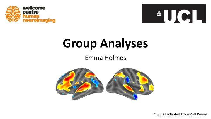
Group Analyses Emma Holmes * Slides adapted from Will Penny
First Level: Subject 1 For voxel v in the brain Effect size (c) 4
First Level: Subject 3 For voxel v in the brain Effect size (c) 2
First Level: Subject 12 For voxel v in the brain Effect size (c) 4
Second Level: Group Analysis c Group effect (mean [m]) Between subject variability (stand dev [sb]) = 1.07 Standard error of the mean (SEM) = 2.67 Subject 1 4 Subject 2 3 = sb /sqrt(N) = 0.31 Subject 3 2 Subject 4 1 Subject 5 1 Subject 6 2 Is the effect significant at voxel v? (one-sample t-test) t = m/SEM = 2.67/0.31 = 8.61 p = 10-6 This is called a Random Effects Analysis, because we compare the group effect to the between-subjects variability Subject 7 3 Subject 8 3 Subject 9 3 Subject 10 2 Subject 11 4 Subject 12 4
Second Level: Group Analysis c Group effect (mean [m]) Between subject variability (stand dev [sb]) = 1.07 Standard error of the mean (SEM) = 2.67 Subject 1 4 Subject 2 3 = sb /sqrt(N) = 0.31 Subject 3 2 Subject 4 1 Subject 5 1 Subject 6 2 Is the effect significant at voxel v? (one-sample t-test) t = m/SEM = 2.67/0.31 = 8.61 p = 10-6 ...also known as the SUMMARY STATISTIC approach: We summarise the response of each subject by a single statistic (their effect size) Subject 7 3 Subject 8 3 Subject 9 3 Subject 10 2 Subject 11 4 Subject 12 4
First Level: Subject 1 For voxel v in the brain Root mean square error (GLM fit) Effect size (c) 4 Within subject variability (sw) 0.9
First Level: Subject 3 For voxel v in the brain Effect size (c) 2 Within subject variability (sw) 1.5
First Level: Subject 12 For voxel v in the brain Effect size (c) 4 Within subject variability (sw) 1.1
Fixed Effects Analysis Concatenate timeseries Subject 1 Subject 3 Subject 12 Each measurement is one scan from one subject we now have 600 scans (50 scans in each of 12 subjects) We use this to calculate the average effect
Group Analysis: Fixed Effects sw 0.9 Group effect (mean [m]) Average within subject variability (sw) Standard error of the mean (SEMW) = 2.67 = 1.07 = sw /sqrt(N) = 0.04 Subject 1 Subject 2 1.2 Subject 3 1.5 Subject 4 0.5 Subject 5 0.4 Subject 6 0.7 Subject 7 0.8 Is the effect significant at voxel v? t = m/SEMW = 62.7 p = 10-51 Overconfident? Subject 8 2.1 Number of data points is now total number of scans (i.e. 600) Subject 9 1.8 Subject 10 0.8 Subject 11 0.7 Subject 12 1.1
Random Effects vs. Fixed Effects Fixed Effects Analysis (FFX) We compare the group effect to the within-subject variability. It an inference about this specific sample of subjects. Statistics are often inflated relative to random effects analysis. Random Effects Analysis (RFX) We compare the group effect to the between-subject variability. It is an inference about the population from which the subjects were drawn: If you had a new subject from that population, you could be confident they would also show the effect.
Random Effects vs. Fixed Effects Mixed Effects Analysis (MFX) Has some random and some fixed effects. spm_mfx
Beyond a single voxel Voxel v
Beyond a single voxel Voxel v 0 0 . . . . . . . . . . . . . . . . 0 0 . . . . . . . . . . . . . . . . 0 0 . . . . . . . . . . . . . . . . 0 0 . . . . . . . . . . . . . . . . 0 0 . . . . . . . . . . . . . . . . 0 0 . . . . . . . . . . . . . . . . 0 3 . . . . . . . . . . . . . . . . 2 6 . . . . . . . . . . . . . . . . 4 . . . . . . . . . . . . . . . . 2 4 2 6 . . . . . . . . . . . . . . . . . . 1 1 . . . . . . . . . . . . . . 0 0 . . . . . . . . . . . . . . . . 0 0 . . . . . . . . . . . . . . . . . . . . 0 0 . . . . . . . . . . . .
Random Effects: Summary Statistic First level Data (per voxel) Design Matrix Contrast Image S1 S2 S11 S12
Random Effects: Summary Statistic First level Second level Data (per voxel) Design Matrix Contrast Image One-sample t-test SPM(t) S1 S2 (Thresholded to correct for multiple comparisons) S11 c T c t = ) T ( r a V Random effects: summary statistic approach S12
Hierarchical model = + ) 1 ( ) 1 ( ) 1 ( y X Level 1: Multiple variance components at each level = + ) 1 ( ) 2 ( ) 2 ( ) 2 ( X Level 2: = Q ( ) i C ( ) i ( ) i k k ) 1 = ) + ( ( ( ) ( ) n n n n X k Level n: At each level, the distribution of parameters is dependent on the level above What we don t know: distribution of parameters and variance parameters Friston (2008) Hierarchical models in the brain. PLOS Comp. Bio.
Hierarchical Model ( ) ( ) 1 ( ) 1 = + 1 y X First level Second level ( ) 1 ( ) ( ) 2 ( ) 2 = + 2 X ( ) 1 ) 1 ( 1 X (1) Within subject variance, sw(i) (2) Between subject variance,sb ( ) 2 ( ) 1 ( ) 2 y ( ) 1 ( ) 2 = + ) 1 ( 2 X X + = ) 1 ( 3 X spm_reml
Example Results: Auditory Experiment Summary statistic Separates first and second level estimates Hierarchical model Computationally intensive! Friston et al. (2004) Mixed effects and fMRI studies, Neuroimage
Summary Statistic vs. Hierarchical Model The summary stats approach is exact if, for each session/subject: Within-subject variances are the same First-level design (e.g. number of trials) are the same The summary stats approach is robust against typical violations (SPM book 2006; Mumford and Nichols, 2009, Neuroimage). We might use a hierarchical model in epilepsy research where number of seizures is not under experimental control and is highly variable over subjects.
Beyond the one sample t-test Second level
Multiple Conditions (within subjects) Condition 1 Condition 2 Condition 3 Subject 1 Subject 1 Subject 1 Subject 2 Subject 2 Subject 2 Subject 12 Subject 12 Subject 12 Second level: One-way within-subjects ANOVA
Multiple Conditions (between subjects) Condition 1 Condition 2 Condition 3 Subject 1 Subject 13 Subject 25 Subject 2 Subject 14 Subject 26 Subject 12 Subject 24 Subject 36 e.g., effects of a drug Second level: One-way between-subjects ANOVA (or if only two conditions, a two-sample t-test)
Testing for interactions Within-within interactions: Can be done at the first level (i.e., specify contrasts according to the interaction to be tested) Between-between interactions: Test at the second level Within-between interactions: Specify within-subjects factor(s) at the first level, then the between-subjects factor(s) at the second level
Summary Group inference usually proceeds with random effects analysis, not fixed effects analysis. Group effects are compared to between rather than within subject variability Hierarchical models provide a gold-standard for random effects group analysis, but are computationally intensive Summary statistics are a robust method for random effects group analysis when conditions are met If you want to contrast two conditions within subjects, you can use a one-sample t-test at the second level. If more conditions, you can use a one-way ANOVA. If different groups, you can use a between-subjects ANOVA or two-sample t-test


