Soil Variability and Fertility Management


Soil Variability and Fertility
Management
Chapter 6

•
Among the numerous challenges of crop production is the
management of soil nutrients, soil moisture content and crop and soil
variability. One of the first problems that was addressed in precision
agriculture was site-specific nutrient management (
). Since then, advancements have been made in the
creation of mathematical approaches that can be used to help match
fertilizer recommendations to soil and crop productivity. This chapter
will review sources of soil variability and current management tools
and techniques to help growers manage soil variability.Nowak, 1999Pierce and
S
o
u
r
c
e
s
o
f
S
o
i
l
V
a
r
i
a
b
i
l
i
t
y
•
Variability can result from many factors, including those from inherent
differences produced during soil development, the result of erosion
following tillage, and systematic errors from uneven application of
fertilizers and manures (
Franzen, 2011
). Variability is discussed in
more detail in Chapter 2 (
Kitchen and Clay, 2018
).
G
e
n
e
r
a
l
S
o
i
l
S
a
m
p
l
i
n
g
B
a
s
i
c
s
•
Soil sampling is variable in three dimensions
•
There is two-dimensional variability that is most often considered: forward,
backward, and side to side.
•
But there is also vertical variability.
•
Tillage and lack there-of complicates the Vertical.
•
Banding, No matter depth highly complicates Horizontal.
•
Starter for row crops complicates less.
Watkins et al.
Minimum of 10 years in a no-till management system.
Watkins et al.
Sampling
9 On farm No-till Wheat P Response Studies
Watkins et al.
Watkins et al.
Sampling in Banded Fields.
Fig. 6.1.
Sampling strategy for soil P and K in a transect perpendicular to row direction spanning at least one complete row. Sample
depth could be 6 to 8 inches depending on the sampling depth basis of regional, state, province or state P and K
recommendations.
How we Do Nitrogen – Corn
Option 1:
•
Well, ___________ (fill in name) did it this way.
Option 2:
•
What did __________ (fill in name of guy down
the road that grows good corn) do?
How N is done.
Nitrogen in the Crop - EONR
Stanford Equation
Stanford Equation
Theoretical Equation
Nitrogen in the Crop - EONR
1.67 1.58 .51 .77 1.14 1.36 3.22 2.22 1.33 1.5 1.4
Average of 68 lbs with 49 BPA, 1.5 lbs N per bushel
Fine and Course Control
•
Making high resolution decisions
using low resolution recs.
•
Recommendation maps are at
< 1 acre resolution and critical value
that represents a whole state.
•
How Precise is that.
Where is the opportunity
•
N-Crop: Is the yield Temporally Variable? Spatially Variable?
•
N-Soil: Do you have 2% OM and inconsistent weather?
•
E-Fert - is your texture or landscape spatially variable?
•
Can you adjust based on Management.
How we Do Phosphorus
Soil Testing
was the basis
Determine immediately and potentially available P.
Relate back to Correlation Calibration work. (50s-60s)
“Critical” Values Est.
How we Do Phosphorus Recs
•
Sufficiency program
Feed the Plant
•
Intended to estimate the
long-term average amount
of
fertilizer
P required to, on
average, provide optimum
economic return in the year
of application. There is little
consideration for future soil
test values
How we Do Phosphorus Recs
•
Build-Maintain (Replacement)
•
Apply enough P to or K to build soil test values to a target soil test value
over a planned timeframe (e.g. 4-8 years), then maintain based on crop
removal and soil test levels
•
NOT intended to provide optimum economic returns in a given year, but
minimize the probability the P or K will limit crop yields while providing for
near maximum yield potential
How we Do Phosphorus Recs
•
Build-Maintain
(Replacement)
•
Sounds good and makes
sense right.
•
If we are using this
approach.
•
Does rate matter.
Understanding Crop Response to Fertilizer
Low Soil Test Levels
•
Low yields without additional
fertilizer
•
EOR range is narrow
•
Optimum rate is minimally
affected by grain:nutrient price
ratio
L. Haag, Wheat U - 10 Aug 2016 Wichita
Understanding Crop Response to Fertilizer
Medium Soil Test Levels
•
Expected yield without fertilizer
is higher
•
Range of potentially optimal
rates is wider
•
In a single-year decision
framework, EOR is very sensitive
to grain:nutrient price ratio
•
As price ratio
↓
EOR ↑
L. Haag, Wheat U - 10 Aug 2016 Wichita
Understanding Crop Response to Fertilizer
High Soil Test Levels
•
No or minimal response
to added fertilizer
L. Haag, Wheat U - 10 Aug 2016 Wichita
L. Haag, Wheat U - 10 Aug 2016 Wichita
Economics of Accuracy
L. Haag, Wheat U - 10 Aug 2016 Wichita
How we Do VRT Phosphorus Recs
•
How is it done?
•
Soil : Yield : Soil x Yield: Yield : Soil
•
Grid/Zone Sample, Yield Goal 3-5 yr
•
Grid/Zone, Multi Year Yield, 3 yr
•
Grid/Zone, Update Yield each year.
How we Do VRT Phosphorus Recs
•
Equation for soils below optimum is:
P Rec = (Optimum P – Observed P) *16 / build years + Crop Removal
•
For soils test in the optimum range:
Prec = Crop Removal
•
For Soils in High Range
Prec = Crop Removal *(((Optimum P level + 12.5) – observed P)/7.5)
•
This gradually tapers the rec to 0 once we are 12.5 ppm above optimum
•
Optimum Range is 22.5-27.5 ppm for Row Crops , 20-25ppm for cool season grass
and similar, 15-20ppm for Warm Season grass and similar
How we Do VRT Phosphorus Recs
How we Do VRT Phosphorus Recs
•
Likelihood of VRT based on Sufficiency being off is high.
•
Interpolation of P based on grid is a stretch.
•
Yield monitor data has a higher resolution of positional accuracy.
•
Current VRT using a Course Knob to adjust P.
•
If replacement rates are used soil testing is essential
O
r
i
g
i
n
a
l
S
o
i
l
D
e
v
e
l
o
p
m
e
n
t
•
The five soil forming factors (Jenny, 1941) are parent material,
vegetation, climate, topography and time.
•
PM- Internal drainage, deep acidity,
•
In the coastal plains of the eastern United States, the development of
the present coastline has resulted in swirling patterns of sands of
different silt and clay content (Duffera et al., 2007). Soils with less silt
and clay are more susceptible to mid-season drought, while those
with greater silt and clay content are more resistant to drought, due
to their greater water-holding capacity.
Parent material
•
In western North
Dakota, for example,
different soil textures
within a field are
present at different
elevations due to
layers of sandstone or
siltstone (Fig. 6.2). A
soil originating from
sandstone has less
available water when
compared with a soil
originating from a
siltstone.
F
i
g
.
6
.
2
.
L
a
n
d
s
c
a
p
e
i
n
w
e
s
t
e
r
n
N
o
r
t
h
D
a
k
o
t
a
n
e
a
r
H
e
t
t
i
n
g
e
r
.
S
o
i
l
s
w
i
t
h
i
n
a
f
i
e
l
d
c
o
u
l
d
b
e
t
h
e
r
e
s
u
l
t
o
f
w
e
a
t
h
e
r
i
n
g
m
o
r
e
t
h
a
n
o
n
e
s
e
d
i
m
e
n
t
a
r
y
p
a
r
e
n
t
m
a
t
e
r
i
a
l
.
S
a
l
i
n
i
t
y
•
In some soils, areas of high sodium, or sodic, soils are present. The
sodium may originate from sodium-bearing rocks, such as sodium
feldspars in the parental loess materials in south Illinois, or from
shales in North Dakota and South Dakota
•
In the area west of Grand Forks, ND, some sodium-affected soils are
the result of salty artesian systems from deep underground ancient
sea deposits
•
Excessive soil sodium results in a randomization of the soil clays that
greatly reduce water percolation and crop rooting depth. In
lowsodium, higher-calcium soils, clays tend to bind together in
regularly structured micro- and macroaggregates.
E
r
o
s
i
o
n
•
In areas to the east of the North American Great Plains, water erosion
is a major factor impacting long-term sustainability.
•
In shoulder areas and ridge tops, much if not all of the original top
soil has been lost over time. In valley floors, depressions, and toe
slopes, some of the A horizon has been deposited.
•
Productivity of hilltops and slopes is low compared to depressions,
mostly due to the lack of topsoil, which results in increased crusting,
lower water holding capacity, and surface layer presence of high lime,
which was originally capped with high organic matter soils at the
surface, but are now gone and more susceptible to conditions such as
iron deficiency chlorosis and water stress
F
i
g
.
6
.
3
.
A
w
a
g
o
n
i
n
S
o
u
t
h
D
a
k
o
t
a
,
1
9
3
4
,
n
e
a
r
l
y
c
o
v
e
r
e
d
w
i
t
h
e
r
o
d
e
d
t
o
p
s
o
i
l
(
S
o
u
r
c
e
:
U
S
D
A
)
.
A
f
t
e
r
m
a
t
h
o
f
t
o
p
s
o
i
l
e
r
o
s
i
o
n
d
u
e
t
o
w
i
n
d
,
n
o
r
t
h
e
r
n
R
e
d
R
i
v
e
r
V
a
l
l
e
y
,
N
o
r
t
h
D
a
k
o
t
a
e
a
r
l
y
1
9
9
0
s
.
A
.
C
.
C
a
t
t
a
n
a
c
h
,
A
m
e
r
i
c
a
n
C
r
y
s
t
a
l
S
u
g
a
r
,
r
e
t
i
r
e
d
,
i
m
a
g
e
u
s
e
d
w
i
t
h
p
e
r
m
i
s
s
i
o
n
.
S
y
s
t
e
m
a
t
i
c
V
a
r
i
a
b
i
l
i
t
y
•
Application of fertilizers and manures can result in systematic
variability (Fig. 6.4). Systematic variability is non-natural soil variability
due to the activities of human. Examples of systematic variability are
application of fertilizer and/ or manure either too close, resulting in
increased nutrient content in strips in the direction of travel, and
application of fertilizer and/or manure too far between passes,
leaving untreated strips of soil between wider strips of applied
nutrients
S
y
s
t
e
m
a
t
i
c
V
a
r
i
a
b
i
l
i
t
y
F
i
g
.
6
.
4
.
M
a
n
u
r
e
m
i
s
a
p
p
l
i
c
a
t
i
o
n
n
o
r
t
h
w
e
s
t
o
f
F
a
r
g
o
,
N
D
.
S
y
s
t
e
m
a
t
i
c
V
a
r
i
a
b
i
l
i
t
y
KMZ file
S
y
s
t
e
m
a
t
i
c
V
a
r
i
a
b
i
l
i
t
y
S
o
i
l
S
a
m
p
l
i
n
g
S
t
r
a
t
e
g
i
e
s
f
o
r
S
i
t
e
-
S
p
e
c
i
f
i
c
N
u
t
r
i
e
n
t
M
a
n
a
g
e
m
e
n
t
•
The grid sampling philosophy is based
on the assumption that nutrient
levels are random, unrelated to
anything in nature, and should be
sampled without any sampler bias
toward where to place the sample
locations.
•
Zone sampling philosophy assumes
that nutrient levels and the patt erns
in which they appear in a fi eld are
the result of some logical reason.
G
r
i
d
S
a
m
p
l
i
n
g
•
Grid sampling is used and preferred in regions where past fertilization
or manure application has been high. Native fertility levels that tend
to be zone-based have been masked and overwhelmed through past
fertilizer and manure applications. Grid sampling is used when there
is no apparent logical method of dividing a fi eld into relatively
homogeneous areas.
G
r
i
d
S
a
m
p
l
i
n
g
•
Random sampling might be appropriate in
a fi eld with no recent history of
fertilization or manure, such as a
government set-aside program break-out
fi eld or an old pasture to be converted to
cropland.
F
i
g
.
6
.
5
.
R
a
n
d
o
m
s
a
m
p
l
i
n
g
e
x
a
m
p
l
e
.
G
r
i
d
S
a
m
p
l
i
n
g
•
The clustered approach is a type of
random sample that might help
compensate for small-scale variability
and larger-scale variability by
grouping two to three sample core
composites around random points
F
i
g
.
6
.
6
.
R
a
n
d
o
m
c
l
u
s
t
e
r
s
a
m
p
l
i
n
g
e
x
a
m
p
l
e
.
G
r
i
d
S
a
m
p
l
i
n
g
•
Regular systematic was a common grid
sampling approach in the era before GPS
(global positioning system) receivers. This
approach allowed a sampler to use a
vehicle tachometer or even “step off ”
distances to achieve the desired patt ern.
F
i
g
.
6
.
7
.
R
e
g
u
l
a
r
s
y
s
t
e
m
a
t
i
c
g
r
i
d
s
a
m
p
l
i
n
g
e
x
a
m
p
l
e
.
G
r
i
d
S
a
m
p
l
i
n
g
•
A staggered start systematic recognized
that systematic errors in one direction are
possible, and the start and end of each
sampling rank was off set to try to
compensate for these errors in one
direction
F
i
g
.
6
.
8
.
S
t
a
g
g
e
r
e
d
s
t
a
r
t
(
o
r
t
r
i
a
n
g
u
l
a
r
,
o
r
d
i
a
m
o
n
d
)
g
r
i
d
s
a
m
p
l
i
n
g
e
x
a
m
p
l
e
.
G
r
i
d
S
a
m
p
l
i
n
g
•
The systematic unaligned grid was made
practical through a combination of GPS and
field software that would allow random grid
locations within a systematic grid. This
approach minimizes the effects of
systematic errors in two directions. It is also
the method that most supports kriging: the
statistical interpolation method that relates
distance to value estimation between
sampling points. The systematic unaligned
grid is probably the method most used by
commercial grid samplers today.
F
i
g
.
6
.
9
.
S
y
s
t
e
m
a
t
i
c
u
n
a
l
i
g
n
e
d
g
r
i
d
s
a
m
p
l
i
n
g
e
x
a
m
p
l
e
.
Grid Sampling
•
To adequately represent field nutrient levels in fields where the range
of variability is great enough that different recommendation rates of
nutrients are represented, about a sample per acre grid is required
(Franzen and Peck, 1995; Franzen et al., 1998). The expense and time
required for such intensive sampling has led many growers to use a
sampling density less than this, usually one sample per 2.5 acres (1
ha)
Z
o
n
e
S
a
m
p
l
i
n
g
•
Zone sampling strategies were developed in North Dakota and other
states where a more con-servative approach to fertilization has
historically been used due to the high frequency of crop fail-ure due
to drought, and to a lesser extent, floods. In these areas, patterns of
fertility, particularly for residual soil nitrate but also for P, K, soil pH
and other nutrients, are stable over time. The levels for particular
nutrients may increase or decrease over time, but the patterns they
form in the fields are remarkably stable.
Z
o
n
e
S
a
m
p
l
i
n
g
•
A number of tools are available to delineate nutrient management
zones: topogra-phy, satellite imagery, aerial imagery, soil electrical
conductivity (EC) sensors, soil electromagnetic sensors (EM), and
multiyear yield maps (Franzen, 2008). The use of NRCS–published soil
survey boundaries is highly discouraged, because most only depict
polygons over 2.5 acres (1 ha) size, and soils change over time.
Unfortunately, this is often the first ‘tool’ that some use to define
zones because they are easy to access; however, they should not be
used unless the polygons in the soil survey match well with
boundaries defined by some of the tools mentioned previously
(Franzen et al., 2002).
T
o
p
o
g
r
a
p
h
y
•
Within fields, topography influences crop pro-ductivity and nutrient
availability to crops. The obvious affect is the thickness of A-horizon
(the organic rich layer at the soil surface).
•
Nitrogen management is greatly affected by topography and the
texture of parent material. Nitrogen in the form of nitrate is affected
by two important processes: leaching and denitrifica-tion. Soils with a
high leaching potential tend to be loamy texture or sandier, on higher
landscape positions. Soils with high denitrification potential tend to
have a greater clay content in lower land-scape positions.
Topography
F
i
g
.
6
.
1
0
.
“
L
e
v
e
l
”
e
l
e
v
a
t
i
o
n
i
n
R
e
d
R
i
v
e
r
V
a
l
l
e
y
o
f
N
o
r
t
h
D
a
k
o
t
a
.
S
e
v
e
r
e
i
r
o
n
d
e
f
i
c
i
e
n
c
y
c
h
l
o
r
o
s
i
s
i
s
l
o
c
a
t
e
d
o
n
“
b
u
m
p
s
”
i
n
t
h
e
l
a
n
d
s
c
a
p
e
,
w
h
e
r
e
c
e
n
t
u
r
i
e
s
o
f
s
u
m
m
e
r
u
p
w
a
r
d
w
a
t
e
r
m
o
v
e
m
e
n
t
h
a
s
r
e
s
u
l
t
e
d
i
n
a
c
c
u
m
u
l
a
t
e
d
l
i
m
e
a
n
d
s
o
l
u
b
l
e
s
a
l
t
s
.
G
r
e
e
n
e
r
a
r
e
a
s
a
r
e
l
e
a
c
h
e
d
o
f
l
i
m
e
a
n
d
s
a
l
t
s
.
I
m
a
g
e
r
y
•
Satellite imagery quality and pixel size have improved during the past
twenty years. Where LandSat satellites once provided pixels about
100 ft2 (30 m), newer satellites in an affordable context provide 10 to
15 ft2 (3 to 5 m). Additional satellites provide even greater resolution;
however, these have not provided additional nutrient boundary
definition and result in more confusion of pat-terns than firm
definition. Satellite imagery has the advantage of obtaining large
tracts in a single image. However, satellite imagery always has the
disadvantage of cloud interference (Bu et al., 2017).
I
m
a
g
e
r
y
•
Aerial imagery from aircraft has been used for many years to identify
problems in fields. For use in zone delineation, aerial imagery that
data can be collected on cloudy days. However, this is also a
disadvantage in that image contains cloud shadows. The extent of the
image depends on the altitude of the aircraft. At an altitude of 5000 ft
(1500 m), about 160 acres (65 ha) of land can be photographed.
•
UAV’s, unless allowed to operate at the height of aircraft, are forced
to take a series of images that are ‘stitched’ together. The images may
be obtained several minutes of time apart, and different sun angles
may confound the final imagery.
E
l
e
c
t
r
i
c
a
l
C
o
n
d
u
c
t
i
v
i
t
y
•
Soil clay content, moisture content, nutrient lev-els and soluble salts
contribute to different electrical conductivity (EC) readings. A popular
EC detector is manufactured by Veris Technologies (Salinas, KS). It
uses a series of coulters, with electrodes at one of the edge coulters
and one internal to send an electrical signal through the soil, which
arcs through the soil and is detected in another coulter electrode,
provid-ing a ‘shallow’ EC reading and ‘deep’ EC reading in a single
pass through the field (Fig. 6.11).
E
l
e
c
t
r
i
c
a
l
C
o
n
d
u
c
t
i
v
i
t
y
•
The coulters are in contact with the
soil during readings, and the soil
needs sufficient moisture to allow
the electrical signal to travel from
one coulter to another. In some
regions, the EC readings are directly
related to a single soil trait. In
regions of low soluble salt content,
the instrument can be used to
estimate soil clay content, which is
useful in predicting crop pro-
ductivity potential (Sudduth et al.,
2005). In other regions, including
North Dakota, soil clay, moisture,
and soluble salts are present
independently of each other.
F
i
g
.
6
.
1
1
.
V
e
r
i
s
T
e
c
h
n
o
l
o
g
i
e
s
s
o
i
l
E
C
s
e
n
s
o
r
.
C
o
u
r
t
e
s
y
o
f
V
e
r
i
s
T
e
c
h
n
o
l
o
g
i
e
s
,
S
a
l
i
n
a
s
,
K
S
.
E
l
e
c
t
r
o
m
a
g
n
e
t
i
c
S
e
n
s
o
r
s
•
Electromagnetic (EM) sensors measure the capacity to measure
changes in the soils ability to conduct and accumulate electrical
charge (Chapter 9; Adamchuk et al., 2018). In physics, electricity and
magnetism are mathematically related, thus enabling the use of
either one for a similar purpose. Electomagnetic sensors have been
used to map the depth of a clay limiting layer in Missouri. It is also a
zone delineation tool, producing zone maps similar to those
developed using the EC sensor.
E
l
e
c
t
r
o
m
a
g
n
e
t
i
c
S
e
n
s
o
r
s
•
The EM sensors can also be
used in fields with rocks
without harm to the sensor
(Fig. 6.12).
F
i
g
.
6
.
1
2
.
E
M
-
3
8
s
e
n
s
o
r
,
a
n
d
e
l
e
c
t
r
o
m
a
g
n
e
t
i
c
s
e
n
s
o
r
,
c
o
u
r
t
e
s
y
o
f
G
e
o
n
i
c
s
,
L
t
d
.
,
M
i
s
s
i
s
s
a
u
g
a
,
O
N
.
M
u
l
t
i
y
e
a
r
Y
i
e
l
d
M
a
p
s
•
To be most useful, several years of yield maps should be integrated
into a multiyear yield map (Franzen et al., 2008; Chapter 5, Fulton et
al., 2018). Whether a fi eld has had a history of a sin-gle crop or a
diverse crop rotation, the same general procedure should be followed
to create the multiyear yield map. A fi eld that has been in continuous
wheat might average 80 bushels per acre (5 Mg ha-1) one year and 20
bushels per acre (1.2 Mg ha-1) another year. The actual bushels for
the fi eld therefore cannot be used when the data sets are combined.
M
u
l
t
i
y
e
a
r
Y
i
e
l
d
M
a
p
s
•
Standardization is a simple mathematical exer-cise that converts
bushels per acre into relative yield. In the example year of high wheat
yield with high-est yield of 80 bushels per acre (5 Mg ha-1), divide
each yield by 80. The range of yield is then 0 to 1. If the next year is
canola, and the highest canola yield was 3500 pounds per acre, divide
each yield by 3500. The range of yield is from 0 to 1.
F
i
g
.
6
.
1
3
.
A
m
u
l
t
i
y
e
a
r
y
i
e
l
d
m
a
p
o
f
c
o
r
n
a
n
d
s
o
y
b
e
a
n
r
o
t
a
t
i
o
n
s
i
n
a
4
0
-
a
c
r
e
f
i
e
l
d
n
e
a
r
T
h
o
m
a
s
b
o
r
o
,
I
L
,
o
v
e
r
4
y
r
.
Y
i
e
l
d
f
r
e
q
u
e
n
c
y
i
s
r
e
l
a
t
i
v
e
y
i
e
l
d
f
r
o
m
t
h
e
m
e
a
n
(
0
)
v
a
l
u
e
.
P
o
s
i
t
i
v
e
v
a
l
u
e
s
a
r
e
i
n
c
r
e
a
s
i
n
g
y
i
e
l
d
o
v
e
r
m
e
a
n
y
i
e
l
d
s
,
w
h
i
l
e
n
e
g
a
t
i
v
e
v
a
l
u
e
s
a
r
e
d
e
c
r
e
a
s
i
n
g
y
i
e
l
d
f
r
o
m
t
h
e
m
e
a
n
.
F
r
o
m
F
r
a
n
z
e
n
,
2
0
0
6
.
C
o
m
b
i
n
a
t
i
o
n
s
o
f
Z
o
n
e
M
a
p
p
i
n
g
T
o
o
l
s
•
Management zone soil nutrient maps are often based on elevation, soil
nutrient levels, crop reflec-tance, EC, and yield maps (Franzen et al., 2011).
These maps can be produced by first producing individual zone maps of
each tool database for the field. A layering program then is used to
superim-pose the value and location of each zone map pixel geographically
over the corresponding pixel of the other zone map(s). A clustering
program then is used to analyze the patterns from each zone map to
produce the final multi-zone map. An example of this approach is available
in Clay et al. (2017).
•
The choice of zone number is largely left to the consultant or grower.
Usually three to five zones for fields from 40 acres (16.1 ha) to 640 acres
(259 ha) are selected. Up to 10 zones have been used to man-age fields in
extreme cases.
S
e
l
e
c
t
i
n
g
a
S
o
i
l
S
a
m
p
l
i
n
g
S
t
r
a
t
e
g
y
•
Grid sampling has been most useful for farms that have received large
amounts of fertilizer or manure in the past, which overwhelms any
relic of natural soil nutrient variation. Examples of this are many areas
in Iowa, Illinois and Indiana, where the fertilizer “buildup and
maintenance” approach have resulted in high soil test levels. There is
vari-ability in these fields, but the variability is all in the ‘high’ range,
so the recommendation would be the same. Because of the
uniformity of recommen-dation, a 2.5-acre grid (1 ha) is acceptable in
these fields. If there is high variabililty in the recom-mendation, then
a high sampling density may be required to create an accurate map
(Franzen and Peck, 1995; Mallarino and Wittry, 2004).
S
e
l
e
c
t
i
n
g
a
S
o
i
l
S
a
m
p
l
i
n
g
S
t
r
a
t
e
g
y
•
Zone sampling is most useful for soil nitrate where the fertilizer
recommendation is based on the resid-ual soil nitrate (Morris et al., 2018).
Residual soil nitrate is related to water movement and crop productivity,
which is most often related to topography and natu-ral variation. In areas
where farmers fertilize using a more conservative ‘sufficiency’ approach,
even soil phosphorus and potassium levels are best delineated using a zone
approach. In the sufficiency approach, the farmer fertilizes each crop, and
although rate is linked to soil test level, the goal is to apply the most
profitable fertilizer application in a given year, not to build a soil test level
to a higher fertility status. In Iowa, Mallarino and Wittry (2014) reported
that the grid approach was best for soil phosphorus, while the
management zone approach was better for potas-sium and soil pH
(Mallarino and Wittry, 2004).
S
e
l
e
c
t
i
n
g
a
S
o
i
l
S
a
m
p
l
i
n
g
S
t
r
a
t
e
g
y
•
So what would you do.
Videos
•
Video 6.1.
How can the knowledge of spatial variability facilitate
decision making in fields?
http://bit.ly/spatial-variability
•
Video 6.2.
Why is soil testing better with precision agriculture?
http://bit.ly/soil-testing-better
•
Video 6.3.
Zone sampling vs. grid sampling.
http://bit.ly/zone-
sampling-vs-grid-sampling
•
Video 6.4.
How can yield maps aid with soil
sampling?
http://bit.ly/yield-maps-soil
C
h
a
p
t
e
r
Q
u
e
s
t
i
o
n
s
•
How might field topography influence soil nutrient variability?
•
Name four factors other than topography that might influence natural soil
nutrient variability.
•
Name two factors that might contribute to systematic variability of soil nutrients.
•
Fields where high rates of phosphate and potash fertilizer were applied in a soil
test buildup
•
program would benefit from which site-specific soil sampling strategy for P and K:
grid or zone?
•
Name four possible tools that might be utilized to help delineate soil nutrient
zones.
•
What soil sampling strategy is used most often to avoid systemic soil sampling
errors and why is it more effective than other strategies?
Addressing challenges in crop production involves managing soil nutrients, moisture content, and variability. Precision agriculture techniques offer solutions such as site-specific nutrient management and mathematical approaches for matching fertilizer recommendations. This chapter discusses sources of soil variability and tools to aid growers in managing it effectively.

Download Presentation

Please find below an Image/Link to download the presentation.
The content on the website is provided AS IS for your information and personal use only. It may not be sold, licensed, or shared on other websites without obtaining consent from the author.If you encounter any issues during the download, it is possible that the publisher has removed the file from their server.
You are allowed to download the files provided on this website for personal or commercial use, subject to the condition that they are used lawfully. All files are the property of their respective owners.
The content on the website is provided AS IS for your information and personal use only. It may not be sold, licensed, or shared on other websites without obtaining consent from the author.
E N D
Presentation Transcript
Soil Variability and Fertility Management Chapter 6
Among the numerous challenges of crop production is the management of soil nutrients, soil moisture content and crop and soil variability. One of the first problems that was addressed in precision agriculture was site-specific nutrient management (Pierce and Nowak, 1999). Since then, advancements have been made in the creation of mathematical approaches that can be used to help match fertilizer recommendations to soil and crop productivity. This chapter will review sources of soil variability and current management tools and techniques to help growers manage soil variability.
Sources of Soil Variability Sources of Soil Variability Variability can result from many factors, including those from inherent differences produced during soil development, the result of erosion following tillage, and systematic errors from uneven application of fertilizers and manures (Franzen, 2011). Variability is discussed in more detail in Chapter 2 (Kitchen and Clay, 2018).
General Soil Sampling General Soil Sampling Basics Basics Soil sampling is variable in three dimensions There is two-dimensional variability that is most often considered: forward, backward, and side to side. But there is also vertical variability. Tillage and lack there-of complicates the Vertical. Banding, No matter depth highly complicates Horizontal. Starter for row crops complicates less.
Watkins et al. Minimum of 10 years in a no-till management system.
Watkins et al. Stratification of Soil Phosphorus Avg. 9 site years Stratification of Soil pH Avg. 9 site years P conc. (mg P / kg soil) soil pH 0.00 20.00 40.00 60.00 80.00 4.00 5.00 6.00 7.00 8.00 0 0 5.08 A 5.08 A soil sampling depth (cm) soil sampling depth (cm) 10.16 B 10.16 A pre_P pH 15.24 C 15.24 B 20.32 20.32 25.4 25.4 30.48 C 30.48 D 35.56 35.56
9 On farm No-till Wheat P Response Studies Watkins et al. 100 0-5 cm 5-10 cm 10-15 cm 15-30 cm Range in M3P (ppm) 80 60 40 20 0 1 2 3 4 5 6 7 8 9 Location Sampling Depth cm 0 -5 5 -10 10 -15 15 -30 Mehlich III Extractable P Min Max Mg P kg-1 2.2 41.1 2.9 43.3 2.3 12.7 1.5 5.3 Soil pH Max Year Location Ave Min Ave 11.8 7.3 4.9 2.7 5.9 6.3 6.2 6.6 8.1 8.2 5.2 9.1 6.9 7.3 7.3 7.8 2014 Stillwater
Sampling in Banded Fields. Fig. 6.1. Sampling strategy for soil P and K in a transect perpendicular to row direction spanning at least one complete row. Sample depth could be 6 to 8 inches depending on the sampling depth basis of regional, state, province or state P and K recommendations.
How we Do Nitrogen Corn Option 1: Well, ___________ (fill in name) did it this way. Option 2: What did __________ (fill in name of guy down the road that grows good corn) do?
*Optimum N rate kg ha-1 Source Location Years Time period (0-N) Yield Range High N Yield Range ---- Mg ha-1 ---- 1.6-7.6 2.7-5.6 0.8-5.9 1.4-6.2 6.6-10.9 5.5-7.3 1.7-5.6 3.2-7.4 3.8-8.2 6.2-11.3 5.6-10.2 2.1-7.4 1.9-9.5 3.1-4.9 1.9-6.1 3.3-5.6 4.5-7.2 5.0-6.0 2.1-6.4 2.7-4.4 6.2-8.9 5.0-8.9 1.8-2.6 2.7-4.2 6.4-7.9 2.7-7.4 Min 50 58 81 134 73 5 70 60 23 0 66 35 0 102 69 99 45 90 11 59 69 13 127 36 182 51 62 44 Max 233 235 237 239 193 131 113 199 126 37 111 230 203 178 204 194 182 117 218 116 96 114 233 196 204 160 173 55 Avg. 130 179 165 197 131 84 91 135 69 18 91 128 98 144 124 153 103 104 104 88 83 75 183 142 193 105 120 43 SD 53 51 49 32 49 69 21 50 36 15 23 46 52 30 47 49 71 20 88 40 13 54 45 75 15 77 45 20 Bundy et al. (2011) Bundy et al. (2011) Mallarino and Torres (2006) Mallarino and Torres (2006) Varvel et al. (2007) Jokela et al. (1989) Carroll Jokela et al. (1989) Webster Fenster et al. (1976) Waseca Fenster et al. (1976) Martin A Fenster et al. (1976) Martin B Al Kaisi et al. (2003) Ismail et al. (1994) NT Ismail et al. (1994) CT Rice et al. (1986) NT Rice et al. (1986) CT Stecker et al. (1993) Columbia Stecker et al. (1993) Novelty Stecker et al. (1993) Corning Peterson et al. (1989) Eck (1982) Shapiro et al. (2006) RS 51cm Shapiro et al. (2006) RS 76cm Meisinger et al. (1985) MT Meisinger et al. (1985) PT Gehl et al. (2005) Rossville Gehl et al. (2005) Scandia WI WI IA IA NE MN MN MN MN MN CO KY KY KY KY MO MO MO NE TX NE NE MD MD KS KS 21 9 20 14 5 3 3 5 7 6 3 20 20 15 15 3 3 2 4 2 3 3 4 4 2 2 1958-1983 1984-1997 1979-2003 1985-2010 1995-2005 1982-1984 1982-1984 1970-1975 1970-1976 1971-1976 1998-2000 1998-2000 1970-1990 1970-1985 1970-1985 1988-1990 1988-1990 1989-1990 1983-1986 1977-1978 1996-1998 1996-1998 1974-1977 1974-1977 2001-2002 2001-2002 4.3-8.8 5.7-9.96 5.1-12.4 5.3-12.8 10.4-13.3 7.1-9.1 1.8-8.7 7.1-10.6 4.0-9.6 6.2-12.0 8.3-10.8 5.2-10.9 3.5-10.4 5.7-9.2 5.0-8.8 6.0-10.1 6.7-9.9 8.2-8.5 3.9-10.0 5.6-5.9 9.4-11.1 7.1-11.0 5.8-8.2 5.1-8.1 11.3-12.6 3.8-11.5 Average SD Total 198
Nitrogen in the Crop - EONR *Optimum N rate kg ha-1 Max 239 193 131 113 199 126 37 96 114 204 160 Location Years Time period (0-N) Yield Range High N Yield Range ---- Mg ha-1 ---- Source Min 134 73 5 70 60 23 0 69 13 182 51 Avg. 197 131 84 91 135 69 18 83 75 193 105 SD 32 49 69 21 50 36 15 13 54 15 77 IA NE MN MN MN MN MN NE NE KS KS 14 5 3 3 5 7 6 3 3 2 2 1985-2010 1995-2005 1982-1984 1982-1984 1970-1975 1970-1976 1971-1976 1996-1998 1996-1998 2001-2002 2001-2002 1.4-6.2 6.6-10.9 5.5-7.3 1.7-5.6 3.2-7.4 3.8-8.2 6.2-11.3 6.2-8.9 5.0-8.9 6.4-7.9 2.7-7.4 5.3-12.8 10.4-13.3 7.1-9.1 1.8-8.7 7.1-10.6 4.0-9.6 6.2-12.0 9.4-11.1 7.1-11.0 11.3-12.6 3.8-11.5 Mallarino and Torres (2006) Varvel et al. (2007) Jokela et al. (1989) Carroll Jokela et al. (1989) Webster Fenster et al. (1976) Waseca Fenster et al. (1976) Martin A Fenster et al. (1976) Martin B Shapiro et al. (2006) RS 51cm Shapiro et al. (2006) RS 76cm Gehl et al. (2005) Rossville Gehl et al. (2005) Scandia
Nitrogen in the Crop - EONR 120 Yield (bu ac-1) Economical Opt N Rate 100 80 60 40 20 0 2004 2005 2006 2007 2008 2009 2010 2011 2012 2013 2014 2015 1.67 1.58 .51 .77 1.14 1.36 3.22 2.22 1.33 1.5 1.4 Average of 68 lbs with 49 BPA, 1.5 lbs N per bushel
Fine and Course Control Fine Control Making high resolution decisions using low resolution recs. Recommendation maps are at < 1 acre resolution and critical value that represents a whole state. How Precise is that. Course Control
Where is the opportunity N-Crop: Is the yield Temporally Variable? Spatially Variable? N-Soil: Do you have 2% OM and inconsistent weather? E-Fert - is your texture or landscape spatially variable? Can you adjust based on Management.
How we Do Phosphorus Soil Testing was the basis Determine immediately and potentially available P. Relate back to Correlation Calibration work. (50s-60s) Critical Values Est. 100 % Max Yld 0 10 Soil Test P (Bray P1 or Mehlich-3) 65
How we Do Phosphorus Recs Sufficiency program Feed the Plant Intended to estimate the long-term average amount of fertilizer P required to, on average, provide optimum economic return in the year of application. There is little consideration for future soil test values
How we Do Phosphorus Recs Build-Maintain (Replacement) Apply enough P to or K to build soil test values to a target soil test value over a planned timeframe (e.g. 4-8 years), then maintain based on crop removal and soil test levels NOT intended to provide optimum economic returns in a given year, but minimize the probability the P or K will limit crop yields while providing for near maximum yield potential Crop Harvest unit P in yield Corn Soybean Wheat Bushel Bushel Bushel .38 .8 .5
How we Do Phosphorus Recs Build-Maintain (Replacement) Sounds good and makes sense right. Build-up maintain fertilizer scheme suggested by the Ohio State University. If we are using this approach. Does rate matter. Nutrient response curve based on soil test, Rutgers Cooperative Extension.
Understanding Crop Response to Fertilizer Low Soil Test Levels Low yields without additional fertilizer EOR range is narrow Optimum rate is minimally affected by grain:nutrient price ratio L. Haag, Wheat U - 10 Aug 2016 Wichita
Understanding Crop Response to Fertilizer Medium Soil Test Levels Expected yield without fertilizer is higher Range of potentially optimal rates is wider In a single-year decision framework, EOR is very sensitive to grain:nutrient price ratio As price ratio EOR L. Haag, Wheat U - 10 Aug 2016 Wichita
Understanding Crop Response to Fertilizer High Soil Test Levels No or minimal response to added fertilizer L. Haag, Wheat U - 10 Aug 2016 Wichita
EXAMPLE OF THE RELATIONSHIP BETWEEN NUMBER OF SOIL CORES PER COMPOSITE SAMPLE AND ERROR 14 13 CONFIDENCE INTERVAL (+- ppm P) 12 11 MEAN SOIL P = 19ppm 10 9 8 7 6 5 4 3 2 1 0 0 5 10 15 20 25 30 35 40 45 50 NUMBER OF CORES PER SAMPLE L. Haag, Wheat U - 10 Aug 2016 Wichita
Economics of Accuracy L. Haag, Wheat U - 10 Aug 2016 Wichita
How we Do VRT Phosphorus Recs How is it done? Soil : Yield : Soil x Yield: Yield : Soil Grid/Zone Sample, Yield Goal 3-5 yr Grid/Zone, Multi Year Yield, 3 yr Grid/Zone, Update Yield each year.
How we Do VRT Phosphorus Recs Equation for soils below optimum is: P Rec = (Optimum P Observed P) *16 / build years + Crop Removal For soils test in the optimum range: Prec = Crop Removal For Soils in High Range Prec = Crop Removal *(((Optimum P level + 12.5) observed P)/7.5) This gradually tapers the rec to 0 once we are 12.5 ppm above optimum Optimum Range is 22.5-27.5 ppm for Row Crops , 20-25ppm for cool season grass and similar, 15-20ppm for Warm Season grass and similar
How we Do VRT Phosphorus Recs 180 100 bpa 160 150 BPA 140 200 BPA P2O5 REC (LBS/AC) 120 250 BPA Sufficiency 100 80 60 40 20 0 0 10 20 30 40 50 60 Soil Test P (M3P ppm)
How we Do VRT Phosphorus Recs Likelihood of VRT based on Sufficiency being off is high. Interpolation of P based on grid is a stretch. Yield monitor data has a higher resolution of positional accuracy. Current VRT using a Course Knob to adjust P. If replacement rates are used soil testing is essential
Original Soil Original Soil Development Development The five soil forming factors (Jenny, 1941) are parent material, vegetation, climate, topography and time. PM- Internal drainage, deep acidity, In the coastal plains of the eastern United States, the development of the present coastline has resulted in swirling patterns of sands of different silt and clay content (Duffera et al., 2007). Soils with less silt and clay are more susceptible to mid-season drought, while those with greater silt and clay content are more resistant to drought, due to their greater water-holding capacity.
Parent material In western North Dakota, for example, different soil textures within a field are present at different elevations due to layers of sandstone or siltstone (Fig. 6.2). A soil originating from sandstone has less available water when compared with a soil originating from a siltstone. Fig. 6.2. Landscape in western North Dakota near Hettinger. Soils within a field could be the result of weathering more than one sedimentary parent material.
Salinity Salinity In some soils, areas of high sodium, or sodic, soils are present. The sodium may originate from sodium-bearing rocks, such as sodium feldspars in the parental loess materials in south Illinois, or from shales in North Dakota and South Dakota In the area west of Grand Forks, ND, some sodium-affected soils are the result of salty artesian systems from deep underground ancient sea deposits Excessive soil sodium results in a randomization of the soil clays that greatly reduce water percolation and crop rooting depth. In lowsodium, higher-calcium soils, clays tend to bind together in regularly structured micro- and macroaggregates.
Erosion Erosion In areas to the east of the North American Great Plains, water erosion is a major factor impacting long-term sustainability. In shoulder areas and ridge tops, much if not all of the original top soil has been lost over time. In valley floors, depressions, and toe slopes, some of the A horizon has been deposited. Productivity of hilltops and slopes is low compared to depressions, mostly due to the lack of topsoil, which results in increased crusting, lower water holding capacity, and surface layer presence of high lime, which was originally capped with high organic matter soils at the surface, but are now gone and more susceptible to conditions such as iron deficiency chlorosis and water stress
Fig. 6.3. A wagon in South Dakota, 1934, nearly covered with eroded topsoil (Source: USDA). Aftermath of topsoil erosion due to wind, northern Red River Valley, North Dakota early 1990s. A. C. Cattanach, American Crystal Sugar, retired, image used with permission.
Systematic Systematic Variability Variability Application of fertilizers and manures can result in systematic variability (Fig. 6.4). Systematic variability is non-natural soil variability due to the activities of human. Examples of systematic variability are application of fertilizer and/ or manure either too close, resulting in increased nutrient content in strips in the direction of travel, and application of fertilizer and/or manure too far between passes, leaving untreated strips of soil between wider strips of applied nutrients
Systematic Variability Systematic Variability Fig. 6.4. Manure misapplication northwest of Fargo, ND.
Systematic Variability Systematic Variability
Systematic Variability Systematic Variability
Soil Sampling Strategies for Site Soil Sampling Strategies for Site- -Specific Nutrient Nutrient Management Management Specific The grid sampling philosophy is based on the assumption that nutrient levels are random, unrelated to anything in nature, and should be sampled without any sampler bias toward where to place the sample locations. Zone sampling philosophy assumes that nutrient levels and the patt erns in which they appear in a fi eld are the result of some logical reason.
Grid Grid Sampling Sampling Grid sampling is used and preferred in regions where past fertilization or manure application has been high. Native fertility levels that tend to be zone-based have been masked and overwhelmed through past fertilizer and manure applications. Grid sampling is used when there is no apparent logical method of dividing a fi eld into relatively homogeneous areas.
Grid Sampling Grid Sampling Random sampling might be appropriate in a fi eld with no recent history of fertilization or manure, such as a government set-aside program break-out fi eld or an old pasture to be converted to cropland. Fig. 6.5. Random sampling example.
Grid Sampling Grid Sampling The clustered approach is a type of random sample that might help compensate for small-scale variability and larger-scale variability by grouping two to three sample core composites around random points Fig. 6.6. Random cluster sampling example.
Grid Sampling Grid Sampling Regular systematic was a common grid sampling approach in the era before GPS (global positioning system) receivers. This approach allowed a sampler to use a vehicle tachometer or even step off distances to achieve the desired patt ern. Fig. 6.7. Regular systematic grid sampling example.