Graphical Methods for Data Distributions
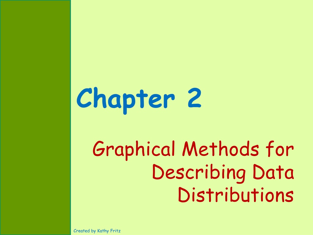

Chapter 2
Graphical Methods for
Describing Data
Distributions

Created by Kathy Fritz


Variable
•
any characteristic whose
value may change
from one individual to another
Political affiliation
Number of textbooks purchased
D
i
s
t
a
n
c
e
f
r
o
m
h
o
m
e
t
o
c
o
l
l
e
g
e


Data
•
The
values
for a variable from
individual
observations
Political affiliation:
Democrat, Republican, etc.
Number of textbooks purchased:
1, 2, 3, 4, . . .
Distance from home to college:
25 miles, 53.5 miles, 347.2 miles, etc.
Suppose that a PE coach records the
height
of each student in his class.
Univariate
– consist of observations on a
single variable
made on individuals in a
sample or population
This is an example of a
univariate
data
Suppose that the PE coach records the
height and weight
of each student in his
class.
Bivariate
- data that consist of pairs of
numbers from
two variables
for each
individual in a sample or population
This is an example of a
bivariate
data
Suppose that the PE coach records the
height, weight, number of sit-ups, and
number of push-ups
for each student in
his class.
Multivariate
-
data that consist of
observations on
two or more variables
This is an example of a
multivariate
data
Two types of variables
categorical
numerical
Categorical variables
•
Qualitative
•
Consist of
categorical
responses
1.
Car model
2.
Birth year
3.
Type of cell phone
4.
Your zip code
5.
Which club you have joined
Which of
these
variables are
NOT
categorical
variables?
They are all
categorical
variables!
Numerical variables
•
quantitative
•
observations or measurements take on
numerical values
1.
GPAs
2.
Height of students
3.
Codes to combination locks
4.
Number of text messages per day
5.
Weight of textbooks
It makes sense to perform math
operations on these values.
Which of these
variables are
NOT
numerical?
Does it makes sense
to find an average
code to combination
locks?
There are two types of
numerical variables -
discrete and continuous
Two types of variables
categorical
numerical
discrete
continuous
Discrete (numerical)
•
Isolated
points along a number line
•
usually
counts
of items
•
Example:
number of textbooks purchased
Continuous (numerical)
•
Variable that can be any value in a
given
interval
•
usually
measurements
of something
•
Example:
GPAs
Identify the following variables:
1.
the color of cars in the teacher’s lot
2.
the number of calculators owned by
students at your college
3.
the zip code of an individual
4.
the amount of time it takes students to
drive to school
5.
the appraised value of homes in your city
Categorical
Categorical
Discrete numerical
Discrete numerical
Continuous numerical
Is money a measurement or a count?
Use the following table to
determine an appropriate
graphical display a data set.
What types of
graphs can be
used with
categorical
data?
In section 2.3, we will
see how the various
graphical displays for
univariate, numerical
data compare.
Displaying
Categorical Data
Bar Charts
Comparative Bar Charts
When to Use:
Univariate, Categorical data
To comply with new standards from the U. S. Department of
Transportation, helmets should reach the bottom of the
motorcyclist’s ears. The report “Motorcycle Helmet Use in 2005 –
Overall Results” (National Highway Traffic Safety Administration,
August 2005) summarized data collected by observing 1700
motorcyclists nationwide at selected roadway locations.
Each time a motorcyclist passed by, the observer noted whether
the rider was wearing no helmet (N), a noncompliant helmet (NC),
or a compliant helmet (C).
The data are summarized in this
table:
Bar Chart
This is called a
frequency distribution
.
A
frequency distribution
is a table that
displays the
possible categories
along
with the
associated frequencies or
relative frequencies
.
The
frequency
for a particular
category is the number of times that
category appears in the data set.
This should equal the
total
number of
observations.
A bar chart is a graphical display for
categorical data.
To compile with new standards from the U. S. Department of
Transportation, helmets should reach the bottom of the
motorcyclist’s ears. The report “Motorcycle Helmet Use in 2005 –
Overall Results” (National Highway Traffic Safety Administration,
August 2005) summarized data collected by observing 1700
motorcyclists nationwide at selected roadway locations.
Each time a motorcyclist passed by, the observer noted whether
the rider was wearing no helmet (N), a noncompliant helmet (NC),
or a compliant helmet (C).
The data is summarized in this
table:
Bar Chart
This should equal
1
(allowing for rounding).
How to construct
1.
Draw a
horizontal
line; write the categories or
labels below the line at regularly spaced
intervals
2.
Draw a
vertical
line; label the scale using
frequency or relative frequency
3.
Place a
rectangular bar
above each category
label with a height determined by its frequency
or relative frequency
Bar Chart
All bars should have the
same width
so
that both the height and the area of
the bar are
proportional
to the
frequency or relative frequency of the
corresponding categories.
What to Look For
Frequently or infrequently occurring
categories
Here is the
completed bar chart
for the motorcycle
helmet data.
Describe this graph.
Bar Chart
Comparative Bar Charts
When to Use
Univariate, Categorical data for
two or more groups
How to construct
•
Constructed by using the
same horizontal and
vertical axes
for the bar charts of two or
more groups
•
Usually
color-coded
to indicate which bars
correspond to each group
•
Should
use
relative frequencies
on the
vertical axis
Bar charts can also be used to provide a visual
comparison of two or more groups.
Why?
You use relative frequency rather
than frequency on the vertical axis
so that you can make
meaningful
comparisons
even if the sample
sizes are not the same.
Each year the Princeton Review conducts a survey of
students applying to college and of parents of college
applicants. In 2009, 12,715 high school students
responded to the question “Ideally how far from home
would you like the college you attend to be?”
Also, 3007 parents of students applying to college
responded to the question “how far from home would
you like the college your child attends to be?” Data is
displayed in the frequency table below.
Create a
comparative
bar chart
with these
data.
What should you do first?
Found by dividing the frequency by the total
number of students
Found by dividing the frequency by the total
number of parents
What does this
graph show about
the ideal distance
college should be
from home?
Displaying
Numerical Data
Dotplots
Stem-and-leaf Displays
Histograms
Dotplot
When to Use
Univariate, Numerical data
How to construct
1.
Draw a
horizontal line
and mark it with an
appropriate numerical scale
2.
Locate each value in the data set along the
scale and
represent it by a dot
. If there are
two are more observations with the same
value,
stack the dots vertically
What to Look For
•
A
representative or typical value (center)
in the data set
•
The extent to which the data values
spread out
•
The
nature of the distribution (shape)
along the number line
•
The presence of
unusual values (gaps and
outliers)
Dotplot
What we look for with
univariate, numerical data
sets are
similar
for
dotplots, stem-and-leaf
displays, and histograms.
An
outlier
is an unusually large or small
data value.
A precise rule for deciding when an observation
is an outlier is given in Chapter 3.
Professor Norm gave a 10-question quiz last
week in his introductory statistics class. The
number of correct answers for each student is
recorded below.
First draw a horizontal line with an
appropriate scale.
The first three observations are
plotted – note that you stack the
points if values are repeated.
This is the completed dotplot.
Write a few
sentence
describing this
distribution.
Professor Norm gave a 10-question quiz last
week in his introductory statistics class. The
number of correct answers for each student is
recorded below.
What to Look For
•
The representative or typical value (center) in the data set
•
The extent to which the data values spread out
•
The nature of the distribution (shape) along the number line
•
The presence of unusual values
The center for the distribution of the number of
correct answers is about 6.
What to Look For
•
The representative or typical value (center) in the data set
•
The extent to which the data values spread out
•
The nature of the distribution (shape) along the number line
•
The presence of unusual values
The center for the distribution of the number of
correct answers is about 6. There is not a lot of
variability in the observations.
What to Look For
•
The representative or typical value (center) in the data set
•
The extent to which the data values spread out
•
The nature of the distribution (shape) along the number line
•
The presence of unusual values
The center for the distribution of the number of
correct answers is about 6. There is not a lot of
variability in the observations. The distribution
is approximately symmetrical with no unusual
observations.
A
symmetrical
distribution is one that has a
vertical line of symmetry where the left half is
a mirror image of the right half.
If we draw a curve,
smoothing out this
dotplot, we will see that
there is
ONLY one peak
.
Distributions with a single
peak are said to be
unimodal
.
Distributions with two
peaks are
bimodal
, and
with more than two peaks
are
multimodal
.
When to Use
Univariate, numerical data with
observations from 2 or more groups
How to construct
•
Constructed using the
same numerical scale
for two or more dotplots
•
Be sure to
include group labels
for the
dotplots in the display
What to Look For
Comment on the same four attributes, but
comparing
the dotplots displayed.
Comparative Dotplots
In another introductory statistics class,
Professor Skew also gave a 10-question quiz. The
number of correct answers for each student is
recorded below.
Create a
comparative
dotplot with the data
sets from the two statistics classes,
Professors’ Norm and Skew.
Write a few
sentences
comparing these
distributions.
The center of the distribution for the number
of correct answers on Prof. Skew’s class is
larger
than the center of Prof. Norm’s class.
There is also
more
variability in Prof. Skew’s
distribution. Prof. Skew’s distribution
appears to have an
unusual observation
where
one student only had 2 answers correct while
there were no unusual observations in Prof.
Norm’s class. The distribution for Prof. Skew
is
negatively skewed
while Prof. Norm’s
distribution is
more
symmetrical.
Is the distribution for Prof. Skew’s class
symmetric? Why or why not?
Notice that the left side (or lower tail) of the
distribution is longer than the right side (or upper tail).
This distribution is said to be
negatively skewed
(or
skewed to the left
).
Distributions where the right tail is longer
than the left is said to be
positively skewed
(or
skewed to the right
).
The
direction of skewness
is always in the
direction of the
longer tail
.
When to Use
Univariate, Numerical data
How to construct
•
Select
one or more of the leading digits
for
the stem
•
List the
possible stem values
in a vertical
column
•
Record the leaf for each observation
beside the corresponding stem
value
•
Indicate the
units for stems and leaves
someplace in the display
Stem-and-Leaf Displays
Stem-and-leaf displays are an effective way to
summarize univariate numerical data when the
data set is not too large
.
Each observation is split into two parts:
Stem
– consists of the first digit(s)
Leaf
-
consists of the final digit(s)
Be sure to list
every stem from
the smallest to the
largest value
What to Look For
•
A
representative or typical value (center)
in the data set
•
The extent to which the data values
spread out
•
The presence of
unusual values (gaps and
outliers)
•
The
extent of symmetry
in the data
distribution
•
The
number and location of peaks
Stem-and-Leaf Displays
The article “Going Wireless” (AARP Bulletin, June
2009) reported the estimated percentage of
households with only wireless phone service (no
landline) for the 50 U.S. states and the District of
Columbia. Data for the
19 Eastern states
are given
here.
What is the variable
of interest?
Wireless percent
A
stem-and-leaf display
is an appropriate way
to summarize these data.
(A dotplot would also be a reasonable choice.)
Let 5.6% be represented as 05.6% so that all the
numbers have two digits in front of the decimal. If we
use the 2-digits, we would have stems from 05 to 20 –
that’s way too many stems!
So let’s just use the first digit (tens) as our stems.
So the leaf will be the last
two digits.
With 05.6%, the leaf is 5.6
and it will be written behind
the stem 0. For the second
number, 5.7 also is written
behind the stem 0 (with a
comma between).
What is the leaf for 20.0%
and where should that leaf be
written?
The completed stem-and-leaf display is shown
below.
However, it is somewhat difficult to read due to
the 2-digit stems.
A common practice is to
drop all but the first digit
in the leaf.
This makes the display
easier to read, but
DOES NOT
change the
overall distribution of
the data set.
The article “Going Wireless” (AARP Bulletin, June
2009) reported the estimated percentage of
households with only wireless phone service (no
landline) for the 50 U.S. states and the District of
Columbia. Data for the
19 Eastern states
are given
here.
While it is not
necessary to write
the leaves in order
from smallest to
largest, by doing so,
the center of the
distribution is more
easily seen.
Write a few
sentences describing
this distribution.
The center of the distribution
for the estimated percentage
of households with only wireless
phone service is approximately
11%. There does not appear to
be much variability. This
display appears to be a
unimodal, symmetric
distribution with no outliers.
Comparative Stem-and-Leaf Displays
When to Use
Univariate, numerical data with
observations from 2 or more group
How to construct
•
List the leaves for one data set to the
right
of the stems
•
List the leaves for the second data set to the
left
of the stems
•
Be sure to
include group labels
to identify
which group is on the left and which is on the
right
The article “Going Wireless” (AARP Bulletin, June
2009) reported the estimated percentage of
households with only wireless phone service (no
landline) for the 50 U.S. states and the District of
Columbia. Data for the
13 Western states
are given
here.
Create a comparative stem-
and-leaf display comparing the
distributions of the Eastern
and Western states.
Write a few
sentences
comparing these
distribution.
The center of the distribution of the estimated
percentage of households with only wireless phone service
for the Western states is a little larger than the center
for the Eastern states. Both distributions are
symmetrical with approximately the same amount of
variability.
When to Use
Univariate numerical data
How to construct
Discrete data
•
Draw a
horizontal
scale and mark it with the possible
values for the variable
•
Draw a
vertical
scale and mark it with frequency or
relative frequency
•
Above each possible value, draw a rectangle
centered
at that value with a height corresponding to its
frequency or relative frequency
What to look for
C
enter
or typical value;
spread
; general
shape
and location and number of peaks; and gaps or
outliers
Constructed differently for
discrete versus continuous
data
Histograms
Dotplots and stem-and-leaf displays
are
not
effective ways to summarize numerical
data when the data
set contains a large
number
of data values.
Histograms
are displays that don’t work
well for small data sets but
do work well
for
larger numerical data sets
.
Discrete numerical data almost
always result from counting. In
such cases, each observation is a
whole number
Queen honey bees mate shortly after they become adults.
During a mating flight, the queen usually takes multiple
partners, collecting sperm that she will store and use
throughout the rest of her life.
A paper, “The Curious Promiscuity of Queen Honey Bees”
(Annals of Zoology [2001]: 255-265), provided the
following data on the number of partners for 30 queen
bees.
12
2
4
6
6
7
8
7
8 11
8
3
5
6
7
10
1
9
7 6
9
7
5
4
7
4
6
7
8 10
Here is a dotplot
of these data.
Queen honey bees continued
Frequency
Number of partners
The variable, number of partners, is discrete. To
create a histogram:
we already have a horizontal axis –
we need to add a vertical axis for frequency
The bars should be
centered
over the
discrete data values and have heights
corresponding to the frequency
of each
data value.
In practice, histograms for discrete data
ONLY
show the
rectangular bars. We built the histogram on top of the
dotplot to show that the
bars are centered
over the
discrete data values and that
heights of the bars are
the frequency
of each data value.
The distribution for the number of partners of queen
honey bees is approximately symmetric with a center
at 7 partners and a somewhat large amount of
variability. There doesn’t appear to be any outliers.
What do you notice about the shapes of
these two histograms?
Here are two histograms showing the
“queen bee data set”. One uses frequency
on the vertical axis, while the other uses
relative frequency
When to Use
Univariate numerical data
How to construct
Continuous data
•
Mark the boundaries of the class intervals on the
horizontal axis
•
Use either frequency or relative frequency on the
vertical axis
•
Draw a rectangle for each class interval directly above
that interval. The height of each rectangle is the
frequency or relative frequency of the corresponding
interval
What to look for
C
enter
or typical value;
spread
; general
shape
and
location and number of peaks; and gaps or
outliers
Histograms with equal width intervals
Consider the following data on carry-on luggage
weight for 25 airline passengers.
Here is a dotplot of this data set.
This is a continuous numerical data set.
With continuous data, the rectangular bars cover
an
interval of data values
(not just one value).
Looking at this dotplot, it is easy to see that we
could use intervals with a width of 5.
This interval includes 10 and all values up to but not
including 15. The next intervals will include 15 and
all values up to but not including 20, and so on.
The top dotplot shows all the data
values in each interval stacked in
the middle of the interval.
From the dotplot, it is easy to see how the
continuous histogram is created.
•
Must use two separate histograms with the
same horizontal axis and relative frequency on
the vertical axis
Comparative Histograms
The article “Early Television Exposure and
Subsequent Attention Problems in Children”
(Pediatrics, April 2004) investigated the television
viewing habits of U.S. children. These graphs show
the viewing habits of 1-year old and 3-year old
children.
The biggest difference between the two histograms
is at the low end, with a much higher proportion of 3-
year-old children falling in the 0-2 TV hours interval
than 1-year-old children.
Histograms with unequal width intervals
When to use
when you have a concentration of data in the
middle with some extreme values
How to construct
construct similar to histograms with
continuous
data, but with
density
on the
vertical axis
When people are asked for the values such as age or weight,
they sometimes shade the truth in their responses. The
article “Self-Report of Academic Performance” (
Social
Methods and Research
[November 1981]: 165-185) focused
on SAT scores and grade point average (GPA). For each
student in the sample, the difference between reported GPA
and actual GPA was determined. Positive differences
resulted from individuals reporting GPAs larger than the
correct value.
When using relative frequency on the vertical axis,
the
proportional area principle is violated
.
Notice the relative frequency for the interval 0.4 to
< 2.0 is
smaller
than the relative frequency for the
interval -0.1 to < 0, but the area of the bar is
MUCH
larger.
GPAs continued
To fix this problem, we
need to find the
density of each
interval.
This is a correct
histogram with unequal
widths.
Cumulative Relative Frequency Plots
When to use
when you want to show the approximate proportion of
data at or below any given value
How to construct
1.
Mark the
boundaries of the class intervals
on a horizontal
axis
2.
Add a
vertical axis
with a scale that goes from 0 to 1
3.
For each class interval, plot the point that is represented by
(upper endpoint of interval, cumulative relative frequency)
4.
Add the point to represented by
(lower endpoint of first interval, 0)
5.
Connect
consecutive points
in the display with line segments
Cumulative Relative Frequency Plots
What to Look For
Proportion of data falling
at or below
any given value along
the
x
axis
The
cumulative relative frequency
of a
given
interval is the
sum
of the current
relative frequency
and all the previous
relative frequencies.
The National Climatic Data Center has been collecting
weather data for many years. A frequency distribution
for annual rainfall totals for Albuquerque, New Mexico,
from 1950 to 2008 are shown in the table below.
0.052
0.155
+
0.792
+
0.999
0.947
0.895
0.516
0.585
0.241
0.344
relative frequency
=
frequency/58
Cumulative relative frequency
=
Current r
elative frequency
+
Previous
relative frequency
The National Climatic Data Center has been collecting
weather for many years. The frequency of the annual
rainfall totals for Albuquerque, New Mexico, from 1950
to 2008 are shown in the table below.
0.052
0.155
0.792
0.999
0.947
0.895
0.516
0.585
0.241
0.344
To create the
cumulative relative frequency plot
:
Plot the
point
(upper value of the interval, cumulative
relative frequency of the interval)
Plot the point:
(smallest value
of the first interval, 0)
The National Climatic Data Center has been collecting
weather for many years. The annual rainfall data for
Albuquerque, New Mexico, from 1950 to 2008, was used
to construct the cumulative relative frequency plot below.
What percent of the years
had rainfall 7.5 inches or
less?
About 30%
Which interval has the
most observations in it,
9 to < 10 or 10 to < 11?
Why?
10 to < 11, because it has a
steeper slope
Displaying Bivariate
Numerical Data
Scatterplots
Time Series Plots
When to Use
Bivariate Numerical data
How to construct
1.
Draw horizontal and vertical axes. Label the
horizontal axis and include an
appropriate scale
for
the
x
-variable. Label the vertical axis and include
an
appropriate scale
for the
y
-variable.
2.
For each (
x
,
y
) pair in the data set, add a dot in
the
appropriate location
in the display.
What to look for
Relationship between
x
and
y
Scatterplots
The accompanying table gives the cost (in
dollars) and an overall quality rating for 10
different brands of men’s athletic shoes
(www.consumerreports.org).
Is there a relationship between
x
= cost and
y
= quality rating?
A scatterplot can help
answer this question
First, draw and label
appropriate horizontal
and vertical axes.
Next, plot each (
x
,
y
) pair.
Here is the completed
scatterplot.
Is there a relationship
between
x
= cost and
y
= quality rating?
There appears to be a
negative relationship
between cost of athletic
shoes and their quality
rating – does that
surprise you?
When to Use
Bivariate data with time and
another variable
How to construct
1.
Draw horizontal and vertical axes. Label the
horizontal axis and include an
appropriate scale
for the
x
-variable. Label the vertical axis and
include an
appropriate scale
for the
y
-variable.
2.
For each (
x
,
y
) pair in the data set, add a dot in
the
appropriate location
in the display.
3.
Connect each dot in order
What to look for
trends or patterns over time
Time Series Plots
The Christmas Price Index is computed each year by
PNC Advisors. It is a humorous look at the cost of
giving all the gifts described in the popular Christmas
song “The Twelve Days of Christmas”
(www.pncchristmaspriceindex.com).
Describe any
trends or
patterns
that you see.
Why is there a downward
trend between 1993 & 1995?
Graphical Displays
in the Media
Pie Charts
Segmented Bar Charts
Pie (Circle) Chart
When to Use
Categorical data
How to construct
•
A circle is used to represent the
whole data set
.
•
“
Slices
” of the pie represent the
categories
•
The size of a particular category’s slice is
proportional
to its frequency or relative
frequency.
•
Most effective for summarizing data sets when
there are not too many categories
Pie (Circle) Chart
The article “Fred Flintstone, Check Your Policy” (
The Washington
Post
, October 2, 2005) summarized a survey of 1014 adults
conducted by the Life and Health Insurance Foundation for
Education. Each person surveyed was asked to select which of five
fictional characters had the greatest need for life insurance:
Spider-Man, Batman, Fred Flintstone, Harry Potter, and Marge
Simpson. The data are summarized in the pie chart.
The survey results were quite
different from the assessment
of an insurance expert.
The insurance expert felt that
Batman, a wealthy bachelor, and
Spider-Man did not need life
insurance as much as
Fred
Flintstone
, a married man with
dependents!
Segmented (or Stacked) Bar Charts
When to Use
Categorical data
How to construct
•
Use a
rectangular bar
rather than a circle
to represent the entire data set.
•
The bar is
divided into segments
, with
different segments representing
different categories.
•
The area of the segment is
proportional to
the relative frequency
for the particular
category.
A pie chart can be difficult to construct by
hand. The circular shape sometimes makes
if difficult to compare areas for different
categories, particularly when the relative
frequencies are similar.
So, we could use a
segmented bar chart
.
Segmented (or Stacked) Bar Charts
Each year, the Higher Education Research Institute
conducts a survey of college seniors. In 2008,
approximately 23,000 seniors participated in the survey
(“Findings from the 2008 Administration of the College
Senior Survey,” Higher Education Research Institute,
June 2009).
This segmented bar
chart summarizes
student responses to
the question:
“During
the past year, how much
time did you spend
studying and doing
homework in a typical
week?”
Common Mistakes
Avoid these Common Mistakes
1.
Areas should be proportional to frequency,
relative frequency, or magnitude of the
number being represented.
The eye is naturally drawn to
large areas in graphical displays.
Sometimes, in an effort to make
the graphical displays more
interesting, designers lose sight
of this important principle.
Consider this graph (
USA Today
,
October 3, 2002).
By replacing the bars of a bar
chart with milk buckets,
areas are distorted
.
The two buckets for 1980
represent 32 cows, whereas
the one bucket for 1970
represents 19 cows.
Avoid these Common Mistakes
1.
Areas should be proportional to frequency,
relative frequency, or magnitude of the
number being represented.
Another common distortion
occurs when a
third
dimension is added
to bar
charts or pie charts. This
distorts the areas and
makes it much more
difficult to interpret.
Avoid these Common Mistakes
2. Be cautious of graphs with broken axes (axes
that don’t start at 0).
•
The use of broken axes in a scatterplot
does not
result
in a misleading picture of the relationship of bivariate
data.
•
In time series plots, broken axes
can sometimes
exaggerate
the magnitude of change over time.
•
In bar charts and histograms, the vertical axis should
NEVER
be broken. This violates the “proportional
area” principle.
Avoid these Common Mistakes
2. Be cautious of graphs with broken axes (axes
that don’t start at 0).
This bar chart is similar to
one in an advertisement for
a software product designed
to raise student test scores.
Areas of the bars are not
proportional to the
magnitude of the numbers
represented – the area for
the rectangle 68 is more
than three times the area of
the rectangle representing
55!
Avoid these Common Mistakes
3.
Watch out for unequal time spacing in time
series plots.
If observations
over time are not
made at regular
time intervals,
special care must
be taken in
constructing the
time series plot.
Notice that the intervals between observations are
irregular
, yet the points in the plot are equally spaced
along the time axis. This makes it
difficult to assess
the rate of change over time.
Here is a
correct
time series plot.
Avoid these Common Mistakes
4.
Be careful how you interpret patterns in
scatterplots.
Consider the following scatterplot showing the relationship between
the number of Methodist ministers in New England and the amount
of Cuban rum imported into Boston from 1860 to 1940
(Education.com).
r
= .999973
A
strong pattern
in a
scatterplot means that
the two variables
tend to
vary
together in a
predictable way, BUT it
does
not
mean that there
is a
cause-and-effect
relationship.
Does an increase in the number of Methodist
ministers
CAUSE
the increase in imported rum?
Avoid these Common Mistakes
5.
Make sure that a graphical display creates
the right first impression.
Consider the following graph
from USA Today (June 25,
2001). Although this graph
does not violate the
proportional area principle,
the way the “bar” for the
none category is displayed
makes this graph difficult to
read. A quick glance at this
graph may leave the reader
with an incorrect impression.
In this chapter, Kathy Fritz presents graphical methods for describing data distributions. It covers variables, data types (univariate, bivariate, multivariate), categorical and numerical variables, and their characteristics. Understand the distinctions between different types of data and variables, such as qualitative and quantitative. Explore the significance of numerical variables, including discrete and continuous types, and the reason for performing mathematical operations on them. Gain knowledge on how to interpret and visualize data effectively.

Download Presentation

Please find below an Image/Link to download the presentation.
The content on the website is provided AS IS for your information and personal use only. It may not be sold, licensed, or shared on other websites without obtaining consent from the author.If you encounter any issues during the download, it is possible that the publisher has removed the file from their server.
You are allowed to download the files provided on this website for personal or commercial use, subject to the condition that they are used lawfully. All files are the property of their respective owners.
The content on the website is provided AS IS for your information and personal use only. It may not be sold, licensed, or shared on other websites without obtaining consent from the author.
E N D
Presentation Transcript
Chapter 2 Graphical Methods for Describing Data Distributions Created by Kathy Fritz
Variable any characteristic whose value may change from one individual to another College Home
Data The values for a variable from individual observations
Suppose that a PE coach records the height of each student in his class. This is an example of a univariate data Univariate consist of observations on a single variable made on individuals in a sample or population
Suppose that the PE coach records the height and weight of each student in his class. This is an example of a bivariate data Bivariate - data that consist of pairs of numbers from two variables for each individual in a sample or population
Suppose that the PE coach records the height, weight, number of sit-ups, and number of push-ups for each student in his class. This is an example of a multivariate data Multivariate - data that consist of observations on two or more variables
Two types of variables categorical numerical
Categorical variables Qualitative Consist of categorical responses 1. Car model 2. Birth year 3. Type of cell phone 4. Your zip code 5. Which club you have joined Which of these variables are NOT categorical variables? They are all categorical variables!
Numerical variables quantitative There are two types of numerical variables - discrete and continuous It makes sense to perform math operations on these values. observations or measurements take on numerical values Which of these variables are NOT numerical? code to combination locks? 1. GPAs 2. Height of students 3. Codes to combination locks 4. Number of text messages per day 5. Weight of textbooks Does it makes sense to find an average
Two types of variables categorical numerical discrete continuous
Discrete (numerical) Isolated points along a number line usually counts of items Example: number of textbooks purchased
Continuous (numerical) Variable that can be any value in a given interval usually measurements of something Example: GPAs
Identify the following variables: 1. the color of cars in the teacher s lot Categorical 2. the number of calculators owned by students at your college Discrete numerical 3. the zip code of an individual Is money a measurement or a count? Categorical 4. the amount of time it takes students to drive to school 5. the appraised value of homes in your city Continuous numerical Discrete numerical
Graphical Display Variable Type Data Type Purpose Display data distribution Compare 2 or more groups Display data distribution Compare 2 or more groups Display data distribution Compare 2 or more groups Display data distribution Investigate relationship between 2 variables Investigate trend over time Univariate Use the following table to determine an appropriate graphical display a data set. Bar Chart Categorical Comparative Bar Chart Univariate for 2 or more groups Categorical What types of graphs can be used with categorical data? Dotplot Univariate Numerical Comparative dotplot Stem-and-leaf display Comparative stem- and-leaf Univariate for 2 or more groups Numerical Univariate Numerical Univariate for 2 groups Numerical In section 2.3, we will see how the various graphical displays for univariate, numerical data compare. Histogram Univariate Numerical Scatterplot Bivariate Numerical Univariate, collected over time Time series plot Numerical
Displaying Categorical Data Bar Charts Comparative Bar Charts
Bar Chart When to Use: Univariate, Categorical data To comply with new standards from the U. S. Department of Transportation, helmets should reach the bottom of the motorcyclist s ears. The report Motorcycle Helmet Use in 2005 Overall Results (National Highway Traffic Safety Administration, August 2005) summarized data collected by observing 1700 motorcyclists nationwide at selected roadway locations. Each time a motorcyclist passed by, the observer noted whether the rider was wearing no helmet (N), a noncompliant helmet (NC), or a compliant helmet (C). category appears in the data set. This is called a frequency distribution. A bar chart is a graphical display for categorical data. A frequency distribution is a table that displays the possible categories along with the associated frequencies or relative frequencies. The frequency for a particular category is the number of times that Helmet Use N NC C Frequency The data are summarized in this table: This should equal the total number of observations. 731 153 816 1700
Bar Chart To compile with new standards from the U. S. Department of Transportation, helmets should reach the bottom of the motorcyclist s ears. The report Motorcycle Helmet Use in 2005 Overall Results (National Highway Traffic Safety Administration, August 2005) summarized data collected by observing 1700 motorcyclists nationwide at selected roadway locations. Each time a motorcyclist passed by, the observer noted whether the rider was wearing no helmet (N), a noncompliant helmet (NC), or a compliant helmet (C). Relative Frequency 0.430 0.090 0.480 The data is summarized in this table: This should equal 1 (allowing for rounding). Helmet Use Helmet Use N NC C C Frequency 731 153 816 1700 1.000 N NC
Bar Chart How to construct 1. Draw a horizontal line; write the categories or labels below the line at regularly spaced intervals the bar are proportional to the frequency or relative frequency of the corresponding categories. All bars should have the same width so that both the height and the area of 2. Draw a vertical line; label the scale using frequency or relative frequency 3. Place a rectangular bar above each category label with a height determined by its frequency or relative frequency
Bar Chart What to Look For Frequently or infrequently occurring categories Here is the completed bar chart for the motorcycle helmet data. Describe this graph.
Comparative Bar Charts When to Use Univariate, Categorical data for two or more groups comparison of two or more groups. than frequency on the vertical axis so that you can make meaningful comparisons even if the sample sizes are not the same. Bar charts can also be used to provide a visual You use relative frequency rather How to construct Constructed by using the same horizontal and vertical axes for the bar charts of two or more groups Usually color-coded to indicate which bars correspond to each group Shoulduse relative frequencies on the vertical axis Why?
Each year the Princeton Review conducts a survey of students applying to college and of parents of college applicants. In 2009, 12,715 high school students responded to the question Ideally how far from home would you like the college you attend to be? Also, 3007 parents of students applying to college responded to the question how far from home would you like the college your child attends to be? Data is displayed in the frequency table below. What should you do first? Frequency Create a comparative bar chart with these data. Ideal Distance Less than 250 miles 250 to 500 miles 500 to 1000 miles More than 1000 miles Students 4450 3942 2416 1907 Parents 1594 902 331 180
Relative Frequency Students .35 .31 .19 .15 Ideal Distance Less than 250 miles 250 to 500 miles 500 to 1000 miles More than 1000 miles Found by dividing the frequency by the total number of students Found by dividing the frequency by the total number of parents Parents .53 .30 .11 .06 What does this graph show about the ideal distance college should be from home?
Displaying Numerical Data Dotplots Stem-and-leaf Displays Histograms
Dotplot When to Use How to construct 1. Draw a horizontal line and mark it with an appropriate numerical scale Univariate, Numerical data 2. Locate each value in the data set along the scale and represent it by a dot. If there are two are more observations with the same value, stack the dots vertically
Dotplot What to Look For A representative or typical value (center) in the data set The extent to which the data values spread out The nature of the distribution (shape) along the number line The presence of unusual values (gaps and outliers) dotplots, stem-and-leaf displays, and histograms. An outlier is an unusually large or small data value. A precise rule for deciding when an observation is an outlier is given in Chapter 3. What we look for with univariate, numerical data sets are similar for
The first three observations are plotted note that you stack the points if values are repeated. Professor Norm gave a 10-question quiz last week in his introductory statistics class. The number of correct answers for each student is recorded below. First draw a horizontal line with an appropriate scale. This is the completed dotplot. 6 8 6 8 5 7 6 4 6 5 6 6 4 7 6 7 7 5 9 3 5 4 8 9 5 7 Write a few sentence describing this distribution. 2 2 4 4 4 6 6 6 8 8 8 10 10 10 2 Number of correct answers Number of correct answers Number of correct answers
What to Look For The representative or typical value (center) in the data set The extent to which the data values spread out The nature of the distribution (shape) along the number line The nature of the distribution (shape) along the number line vertical line of symmetry where the left half is smoothing out this What to Look For The representative or typical value (center) in the data set The extent to which the data values spread out The nature of the distribution (shape) along the number line The presence of unusual values The presence of unusual values The presence of unusual values a mirror image of the right half. dotplot, we will see that there is ONLY one peak. What to Look For The representative or typical value (center) in the data set The extent to which the data values spread out A symmetrical distribution is one that has a If we draw a curve, Professor Norm gave a 10-question quiz last week in his introductory statistics class. The number of correct answers for each student is recorded below. Distributions with a single peak are said to be unimodal. 2 Number of correct answers 4 6 8 10 The center for the distribution of the number of The center for the distribution of the number of correct answers is about 6. There is not a lot of with more than two peaks are multimodal. The center for the distribution of the number of correct answers is about 6. correct answers is about 6. There is not a lot of variability in the observations. variability in the observations. The distribution is approximately symmetrical with no unusual observations. Distributions with two peaks are bimodal, and
Comparative Dotplots When to Use Univariate, numerical data with observations from 2 or more groups How to construct Constructed using the same numerical scale for two or more dotplots Be sure to include group labels for the dotplots in the display What to Look For Comment on the same four attributes, but comparing the dotplots displayed.
Create a comparative dotplot with the data sets from the two statistics classes, Professors Norm and Skew. Is the distribution for Prof. Skew s class Distributions where the right tail is longer than the left is said to be positively skewed (or skewed to the right). In another introductory statistics class, Professor Skew also gave a 10-question quiz. The number of correct answers for each student is recorded below. symmetric? Why or why not? The direction of skewness is always in the direction of the longer tail. 6 8 8 8 7 7 10 8 6 8 9 6 8 7 6 7 7 5 9 3 5 8 8 9 10 7 8 The center of the distribution for the number of correct answers on Prof. Skew s class is largerthan the center of Prof. Norm s class. There is also morevariability in Prof. Skew s distribution. Prof. Skew s distribution appears to have an unusual observation where one student only had 2 answers correct while there were no unusual observations in Prof. Norm s class. The distribution for Prof. Skew is negatively skewed while Prof. Norm s Prof. Skew Write a few sentences comparing these distributions. distribution is more symmetrical. Notice that the left side (or lower tail) of the distribution is longer than the right side (or upper tail). This distribution is said to be negatively skewed (or skewed to the left). Prof. Norm 2 Number of correct answers 4 6 8 10
Stem-and-Leaf Displays When to Use Univariate, Numerical data How to construct Select one or more of the leading digits for the stem List the possible stem values in a vertical column Record the leaf for each observation beside the corresponding stem value Indicate the units for stems and leaves someplace in the display Stem-and-leaf displays are an effective way to summarize univariate numerical data when the data set is not too large. Each observation is split into two parts: Stem consists of the first digit(s) Leaf - consists of the final digit(s) Be sure to list every stem from the smallest to the largest value
Stem-and-Leaf Displays What to Look For A representative or typical value (center) in the data set The extent to which the data values spread out The presence of unusual values (gaps and outliers) The extent of symmetry in the data distribution The number and location of peaks
iPhone 5 pictures and parts leaked So the leaf will be the last two digits. below. The completed stem-and-leaf display is shown The article Going Wireless (AARP Bulletin, June 2009) reported the estimated percentage of households with only wireless phone service (no landline) for the 50 U.S. states and the District of Columbia. Data for the 19 Eastern states are given here. 5.6 5.7 20.0 16.8 16.5 11.4 16.3 14.0 10.8 7.8 Let 5.6% be represented as 05.6% so that all the numbers have two digits in front of the decimal. If we use the 2-digits, we would have stems from 05 to 20 that s way too many stems! So let s just use the first digit (tens) as our stems. number, 5.7 also is written behind the stem 0 (with a in the leaf. With 05.6%, the leaf is 5.6 and it will be written behind the stem 0. For the second However, it is somewhat difficult to read due to the 2-digit stems. A common practice is to drop all but the first digit comma between). 13.4 20.6 What is the leaf for 20.0% and where should that leaf be written? easier to read, but DOES NOT change the overall distribution of the data set. 10.8 10.8 9.3 5.1 11.6 11.6 8.0 A stem-and-leaf display is an appropriate way to summarize these data. 0.0 0.0, 0.6 0 0 What is the variable of interest? This makes the display 0 1 2 2 2 2 2 0 0 0 0 1 1 1 1 5.6, 5.7 5.6, 5.7 5.6, 5.7, 9.3, 8.0, 7.8, 5.1 6.8, 6.5, 3.4, 0.8, 1.6, 1.4, 6.3, 4.0, 0.8, 0.8, 1.6 6 6 3 0 1 1 6 4 0 0 1 5 5 9 8 7 5 Wireless percent (A dotplot would also be a reasonable choice.)
iPhone 5 pictures and parts leaked The article Going Wireless (AARP Bulletin, June 2009) reported the estimated percentage of households with only wireless phone service (no landline) for the 50 U.S. states and the District of Columbia. Data for the 19 Eastern states are given here. The center of the distribution for the estimated percentage of households with only wireless phone service is approximately 11%. There does not appear to be much variability. This display appears to be a unimodal, symmetric distribution with no outliers. While it is not necessary to write the leaves in order from smallest to largest, by doing so, the center of the distribution is more easily seen. 5 5 9 8 7 5 6 6 3 0 1 1 6 4 0 0 1 0 0 0 0 Stem: tens Leaf: ones Write a few sentences describing this distribution. 0 1 2 2 0 1 5 5 5 7 8 9 0 0 0 1 1 1 3 4 6 6 6
Comparative Stem-and-Leaf Displays When to Use Univariate, numerical data with observations from 2 or more group How to construct List the leaves for one data set to the right of the stems List the leaves for the second data set to the left of the stems Be sure to include group labels to identify which group is on the left and which is on the right
iPhone 5 pictures and parts leaked The article Going Wireless (AARP Bulletin, June 2009) reported the estimated percentage of households with only wireless phone service (no landline) for the 50 U.S. states and the District of Columbia. Data for the 13 Western states are given here. 11.7 18.9 9.0 16.7 21.1 17.7 25.5 16.3 Western States Eastern States 5 5 5 7 8 9 0 0 0 1 1 1 3 4 6 6 6 0 0 Stem: tens Leaf: ones 9 9 8 0 1 2 8 7 6 6 1 1 0 8.0 11.4 22.1 9.2 10.8 5 2 1 Create a comparative stem- and-leaf display comparing the distributions of the Eastern and Western states. The center of the distribution of the estimated percentage of households with only wireless phone service for the Western states is a little larger than the center for the Eastern states. Both distributions are Write a few sentences comparing these distribution. symmetrical with approximately the same amount of variability.
Histograms When to Use Dotplots and stem-and-leaf displays are not effective ways to summarize numerical data when the data set contains a large number of data values. always result from counting. In such cases, each observation is a Univariate numerical data How to construct Draw a horizontal scale and mark it with the possible values for the variable Draw a vertical scale and mark it with frequency or relative frequency Above each possible value, draw a rectangle centered at that value with a height corresponding to its frequency or relative frequency What to look for Center or typical value; spread; general shape and location and number of peaks; and gaps or outliers Discrete data Constructed differently for discrete versus continuous data Discrete numerical data almost Histogramsare displays that don t work well for small data sets but do work well for larger numerical data sets. whole number
Queen honey bees mate shortly after they become adults. During a mating flight, the queen usually takes multiple partners, collecting sperm that she will store and use throughout the rest of her life. A paper, The Curious Promiscuity of Queen Honey Bees (Annals of Zoology [2001]: 255-265), provided the following data on the number of partners for 30 queen bees. 12 8 9 2 3 7 4 5 5 6 6 4 6 7 7 7 10 4 8 1 6 7 9 7 8 11 7 6 8 10 Here is a dotplot of these data. 2 4 6 8 10 12 Number of Partners
The bars should be centered over the discrete data values and have heights Queen honey bees continued corresponding to the frequency of each data value. 6 Frequency 4 2 2 2 4 4 Number of partners 6 6 8 8 10 10 12 12 0 In practice, histograms for discrete data ONLY show the rectangular bars. We built the histogram on top of the dotplot to show that the bars are centered over the discrete data values and that heights of the bars are at 7 partners and a somewhat large amount of The variable, number of partners, is discrete. To create a histogram: we already have a horizontal axis we need to add a vertical axis for frequency the frequency of each data value. variability. There doesn t appear to be any outliers. The distribution for the number of partners of queen honey bees is approximately symmetric with a center
Here are two histograms showing the queen bee data set . One uses frequency What do you notice about the shapes of these two histograms? on the vertical axis, while the other uses relative frequency
Histograms with equal width intervals When to Use How to construct Mark the boundaries of the class intervals on the horizontal axis Use either frequency or relative frequency on the vertical axis Draw a rectangle for each class interval directly above that interval. The height of each rectangle is the frequency or relative frequency of the corresponding interval What to look for Center or typical value; spread; general shape and location and number of peaks; and gaps or outliers Univariate numerical data Continuous data
The top dotplot shows all the data values in each interval stacked in the middle of the interval. Consider the following data on carry-on luggage weight for 25 airline passengers. With continuous data, the rectangular bars cover an interval of data values (not just one value). Looking at this dotplot, it is easy to see that we could use intervals with a width of 5. This interval includes 10 and all values up to but not including 15. The next intervals will include 15 and all values up to but not including 20, and so on. 25.0 28.0 22.4 17.9 31.4 24.9 10.1 20.9 26.4 27.6 33.8 22.0 30.0 27.6 34.5 18.0 21.9 22.7 28.7 19.9 25.3 28.2 20.8 27.8 28.5 Here is a dotplot of this data set. This is a continuous numerical data set.
From the dotplot, it is easy to see how the continuous histogram is created.
Comparative Histograms The article Early Television Exposure and Subsequent Attention Problems in Children (Pediatrics, April 2004) investigated the television viewing habits of U.S. children. These graphs show year-old children falling in the 0-2 TV hours interval than 1-year-old children. The biggest difference between the two histograms is at the low end, with a much higher proportion of 3- Must use two separate histograms with the same horizontal axis and relative frequency on the vertical axis the viewing habits of 1-year old and 3-year old children. 1-yr-olds 3-yr-olds
Histograms with unequal width intervals When to use when you have a concentration of data in the middle with some extreme values How to construct construct similar to histograms with continuous data, but with density on the vertical axis relative frequency for interval density = width interval of
When people are asked for the values such as age or weight, they sometimes shade the truth in their responses. The article Self-Report of Academic Performance (Social Methods and Research [November 1981]: 165-185) focused on SAT scores and grade point average (GPA). For each student in the sample, the difference between reported GPA and actual GPA was determined. Positive differences resulted from individuals reporting GPAs larger than the correct value. Interval -2.0 to < -0.4 0.023 -0.4 to < -0.2 0.055 -0.2 to < 0.1 0.097 -0.1 to < 0 0.210 0 to < 0.1 0.189 0.1 to 0.2 0.139 0.2 to < 0.4 0.116 0.4 to 2.0 0.171 When using relative frequency on the vertical axis, the proportional area principle is violated. Notice the relative frequency for the interval 0.4 to < 2.0 is smaller than the relative frequency for the interval -0.1 to < 0, but the area of the bar is MUCH larger. Class Relative Frequency
GPAs continued Class Interval -2.0 to < -0.4 -0.4 to < -0.2 -0.2 to < 0.1 -0.1 to < 0 0 to < 0.1 0.1 to 0.2 0.2 to < 0.4 0.4 to 2.0 Relative Frequency 0.023 0.055 0.097 0.210 0.189 0.139 0.116 0.171 Width Density To fix this problem, we need to find the density of each interval. 1.6 0.2 0.1 0.1 0.1 0.1 0.2 1.6 0.014 0.275 0.970 2.100 1.890 1.390 0.580 0.107 relative frequency for interval density = width interval of This is a correct histogram with unequal widths.
Cumulative Relative Frequency Plots When to use when you want to show the approximate proportion of data at or below any given value How to construct 1. Mark the boundaries of the class intervals on a horizontal axis 2. Add a vertical axis with a scale that goes from 0 to 1 3. For each class interval, plot the point that is represented by (upper endpoint of interval, cumulative relative frequency) 4. Add the point to represented by (lower endpoint of first interval, 0) 5. Connect consecutive points in the display with line segments
Cumulative Relative Frequency Plots What to Look For Proportion of data falling at or below any given value along the x axis The cumulative relative frequency of a given interval is the sum of the current relative frequency and all the previous relative frequencies.
Cumulative relative frequency = Current relative frequency + The National Climatic Data Center has been collecting weather data for many years. A frequency distribution for annual rainfall totals for Albuquerque, New Mexico, from 1950 to 2008 are shown in the table below. Annual Rainfall (inches) Frequency 4 to < 5 3 5 to < 6 6 6 to < 7 5 7 to < 8 6 8 to < 9 10 9 to < 10 4 10 to < 11 12 11 to < 12 6 12 to < 13 3 13 to < 14 3 relative frequency = frequency/58 Previous relative frequency Relative Cumulative Relative Frequency 0.052 0.155 0.241 0.344 Frequency 0.052 0.103 0.086 0.103 0.172 0.069 0.207 0.103 0.052 0.052 + + 0.516 0.585 0.792 0.895 0.947 0.999
To create the cumulative relative frequency plot: Plot the point: The National Climatic Data Center has been collecting weather for many years. The frequency of the annual rainfall totals for Albuquerque, New Mexico, from 1950 to 2008 are shown in the table below. Annual Rainfall (inches) Frequency 4 to < 5 3 5 to < 6 6 6 to < 7 5 7 to < 8 6 8 to < 9 10 9 to < 10 4 10 to < 11 12 11 to < 12 6 12 to < 13 3 13 to < 14 3 Plot the point (upper value of the interval, cumulative relative frequency of the interval) (smallest value of the first interval, 0) Relative Cumulative Relative Frequency 0.052 0.155 0.241 0.344 Frequency 0.052 0.103 0.086 0.103 0.172 0.069 0.207 0.103 0.052 0.052 0.516 0.585 0.792 0.895 0.947 0.999


")
")