Factor Analysis

Factor analysis is a statistical method used to explore the underlying structure of measurement models. This study aims to apply factor analysis to investigate hopelessness in advanced cancer patients, comparing curative and palliative subpopulations and evaluating the stability of factor structures over time. Learn about the goals, methods, and applications of factor analysis in cancer research.

Download Presentation

Please find below an Image/Link to download the presentation.
The content on the website is provided AS IS for your information and personal use only. It may not be sold, licensed, or shared on other websites without obtaining consent from the author.If you encounter any issues during the download, it is possible that the publisher has removed the file from their server.
You are allowed to download the files provided on this website for personal or commercial use, subject to the condition that they are used lawfully. All files are the property of their respective owners.
The content on the website is provided AS IS for your information and personal use only. It may not be sold, licensed, or shared on other websites without obtaining consent from the author.
E N D
Presentation Transcript
Factor Analysis Liz Garrett-Mayer, PhD Dept of PHS, Division of Biostats & Bioinf Biostatistics Shares Resource, Hollings Cancer Center Cancer Control Journal Club March 3, 2016
Goals of paper 1. See if previously defined measurement model of hopelessness in advanced cancer fits this sample. Confirmatory Factor Analysis. 2. Describe the factor structure in these two subpopulations (curative and palliative). Describe the factor structure in these two subpopulations (curative and palliative). Exploratory Factor Analysis. Exploratory Factor Analysis. 3. 4. Evaluate stability of factor structure: does the factor structure stay the same after 12 months? Confirmatory Factor Analysis.
(Exploratory) Factor Analysis Data reduction tool Removes redundancy or duplication from a set of correlated variables Represents correlated variables with a smaller set of derived variables (aka factors ). Factors are formed that are relatively independent of one another. Two types of variables : latent variables: factors observed variables (aka manifest variables; items)
Examples Diet Air pollution Personality Customer satisfaction Depression Quality of Life Quality of Life
Some Applications of Factor Analysis 1. Identification of Underlying Factors: clusters variables into homogeneous sets creates new variables (i.e. factors) allows us to gain insight to categories 2. Screening of Variables: identifies groupings to allow us to select one variable to represent many useful in regression (recall collinearity) 3. Summary: Allows us to describe many variables using a few factors 4. Clustering of objects: Helps us to put objects (people) into categories depending on their factor scores
Perhaps the most widely used (and misused) multivariate [technique] is factor analysis. Few statisticians are neutral about this technique. Proponents feel that factor analysis is the greatest invention since the double bed, while its detractors feel it is a useless procedure that can be used to support nearly any desired interpretation of the data. The truth, as is usually the case, lies somewhere in between. Used properly, factor analysis can yield much useful information; when applied blindly, without regard for its limitations, it is about as useful and informative as Tarot cards. In particular, factor analysis can be used to explore the data for patterns, confirm our hypotheses, or reduce the Many variables to a more manageable number. -- Norman Streiner, PDQ Statistics
Exploratory Factor Analysis Takes a set of variables thought to measure an underlying latent variable: Determines which ones hang together Identifies how many dimensions there are to the latent variable of interest Determines which are the strongest variables: which ones contain most of the information Which ones might be able to be removed due to either redundancy or because they don t hang with other variables. One of the primary goals of factor analysis is often to identify a measurement model variable This includes : Identifying the items to include in the model Identifying how many factors there are in the latent variable (i.e. the dimensionality of the latent variable). Identifying which items are associated with which factors measurement model for a latent
In our example: Hopelessness as measured by the Beck hopelessness scale
Goals of this EFA What structure is there to hopelessness in these patient populations? Can we come up with components of hopelessness? If so, what do they look like? How do we do this? Factor analysis is PURELY based on the correlation matrix (or covariance matrix) of your items. It searches for commonality among the items based on the correlations Think about it: if the items are all measuring the same traits . The correlation patterns can be used to see which of the items cluster together, which don t and how much of each item is simply noise. Note about Likert scale variables: Very noisy! Correlation matrices are more apt for truly continuous variables.
Graphically, a two factor EFA (with 7 items in the scale) F2 F2 F1 F1 y1 y5 y6 y4 y2 y3 y7
Mathematically, the 2 factor EFA (with 20 items in the scale) = = + + + + x x 11 1 F F F e 1 12 2 1 e i i i i 21 1 F 2 22 2 2 i i i i = 20,1 1 + + x F F e 20, 20,2 2 20, i i i i Interpretations: F1 and F2 are the latent variables (e.g. F1i is the value of the ithperson s F1) The s are called loadings and each one represents, in a loose sense, the correlation between each item from the scale and the factor.
Graphically, a two factor EFA (with 7 items in the scale) 71 12 F2 F2 F1 F1 22 72 32 31 11 21 y1 y5 y6 y4 y2 y3 y7 e1 e5 e6 e3 e7 e4 e2
Some statistical stuff Without additional assumptions, the model would be unidentifiable and also hard to interpret. Assumptions Assumptions: F1 and F2 are statistically independent (uncorrelated) in most implementations F1 and F2 are each normally distributed with mean 0, variance 1 Conditional on the latent variables, the error terms are independent.
Spangenberg Paper Recruited participants as part of a prospective observational study, investigating meaning-focused coping and mental health in cancer patients. 732 eligible adult cancer patients receiving treatment with curative or palliative intention in inpatient and outpatient cancer care facilities in Northern Germany were asked to participate. At baseline, 315 patients participated. At follow-up, 158 could be reassessed at 12 months.
Factor 1 comprises items reflecting mainly pessimistic/resigned beliefs (e.g. Item 12), whereas Factor 2 especially contains items reflecting positive beliefs explicitly referring to the future (e.g. Item 5). It is noteworthy that Factor 2 solely includes positively worded items, whereas Factor 1 includes negatively worded items only. Factor 1 includes Items 2, 9, 12, 14, 16, 17, and 20 (curative sample, Cronbach alpha 0.88; palliative sample, alpha=0.85). Factor 2 includes Items 5, 6, 8, 10, 15 and 19 (alpha=0.73 in both samples). Both factors are moderately correlated (r=0.45)
Lets reverse: why two factors? How do you figure out how many factors? That is, what is the dimensionality dimensionality of the latent variable? For a dataset with, let s say 20 variables, fit a principal components analysis (aka PCA, which is, loosely, a kind of factor analysis). a) The PCA creates a matrix of weights from the data from which you can generate composite variables. b) The weights are chosen so that the 1st component (i.e. a weighted average of the variables) explains the maximum amount of variance in the variables. c) The weights for the 2nd component are chosen to maximize the variance remaining in the data AFTER having already computed the 1st PC d) And so on for the remaining 18 (20 2 = 18) components. What? What? This isn t as abstract as it sounds There are scales out there that use this kind of component or composite variable approach. Example: 0.5x1 + 0.75x2 + x3 = z This approach just finds the optimal weights to maximize the variability explained.
Eigenvalues Each of the principal components (aka eigenvectors) has a corresponding value called an eigenvalue which represents the amount of variability explained by the component the amount of variability explained by the component. The sum of the eigenvalues is equal to the number of variables in your analysis (e.g. for Spangenberg paper, the sum of the eigenvalues is 20). There are several rules of thumb for using the eigenvalues to help determine the number of components or factors to keep. 1. Keep as many components as have eigenvalues greater than 1. 2. use a screeplot to determine how many components to keep. 3. Preset a threshold for percent variance explained and keep enough to explain a sufficient amount of variance. Think about what it means to have an eigenvalue of 1 or greater?
From Spangenberg: Initially, five eigenvalues were >1 in the curative sample (7.42, 2.04, 1.53, 1.25, and 1.01). In the palliative sample, four eigenvalues were >1 (7.13, 1.96, 1.43 and 1.14). The scree plot suggested a two factor structure in both patient groups. Note: THESE SCREE PLOTS ARE INCOMPLETE! Note: THESE SCREE PLOTS ARE INCOMPLETE!
In terms of percent variance explained Divide the eigenvalue by the number of variables in the model and you get the incremental variance explained. You can also calculate cumulative variance of the first, for example, 3 components.
Two factor solution Explains about 50% of the variance in the data. Thus, 50% of the information in the data is discarded when only two components are retained. However, there were TWENTY variables that you started with. And, it s quite possible that there is a lot of noise Likert scale variables How much is noise? How much is signal Glass half-full: With only TWO components, you can explain as much as almost TEN variables (on average).
Pick number of factors Based on the examination of eigenvalues, determine the number of factors you want to retain in a factor analysis. Fit a factor analysis where you pre-specify the number of factors.
Interpretable? The problem with PCA and an unrotated factor analysis is that the factors are hard to interpret. The first component or factor usually has about equal loadings (+/- depending on the direction of the item) for all items. The second component may have some high, some low loading, but usually not very interpretable. Solution? Factor rotation.
Rotation: More statistical stuff In principal components, the first factor describes most of variability. After choosing number of factors to retain, we want to spread variability among factors. spread variability more evenly To do this we rotate factors: redefine factors such that loadings on various factors tend to be very high (-1 or 1) or very low (0) intuitively, it makes sharper distinctions in the meanings of the factors We use factor analysis for rotation NOT principal components! We use factor analysis for rotation NOT principal components!
How can we do this? Doesnt it change our answer ? Statistically, it doesn t. The percent variance is the same, etc. For a factor analysis solution to be calculated, there have to be constraints, or assumptions. Some of them are Factors are normally distributed Factors have mean 0 and variance 1 In the initial solution, another constraint is that the first factor explains the most variance, the 2ndfactor explains the next most conditional on the first factor, etc. What if we change this last assumption and instead create a different constraint to make it identifiable? That is, focus on shrinking loadings?
Rotation types orthogonal : maintains independent factors (i.e uncorrelated factors) oblique : allows some dependence. Usually not terribly different from orthogonal, but loadings are often shrunk more towards 0 or 1 (or -1). Spangenberg assumed that factors would be likely to be correlated, so they used oblique rotation.
Aside Principal factors vs. principal components. The defining characteristic that distinguishes between the two factor analytic models is that in principal components analysis we assume that allvariability in an item should be used in the analysis, while in principal factors analysis we only use the variability in an item that it has in common with the other items. In most cases, these two methods usually yield very similar results. However, principal components analysis is often preferred as a method for data reduction, while principal factors analysis is often preferred when the goal of the analysis is to detect structure. (http://www.statsoft.com/textbook/stfacan.html)
Factor 1 comprises items reflecting mainly pessimistic/resigned beliefs (e.g. Item 12), whereas Factor 2 especially contains items reflecting positive beliefs explicitly referring to the future (e.g. Item 5). It is noteworthy that Factor 2 solely includes positively worded items, whereas Factor 1 includes negatively worded items only. Factor 1 includes Items 2, 9, 12, 14, 16, 17, and 20 (curative sample, Cronbach alpha 0.88; palliative sample, alpha=0.85). Factor 2 includes Items 5, 6, 8, 10, 15 and 19 (alpha=0.73 in both samples). Both factors are moderately correlated (r=0.45)
A few more details Keeping vs. dropping items Should look at the fitted model (before or after rotation) to determine the variable s uniqueness. Communality = 1 Uniqueness Communality is a measure of how much is shared between the item and the latent variable structure Uniqueness is what is left over (i.e. noise) Uniqueness DOES depend on the number of factors retained.
A few more details Estimation
Next steps You can use your model to calculate the estimated factor scores for each subject in your dataset Confirmatory factor analysis: Restrictive approach which forces some of the arrows (i.e. loadings) to be zero. EFA: descriptive approach to determine structure CFS: test a particular structure. Applications?
CFA: compare structure to a fixed model F2 F2 F1 F1 72 42 31 11 52 21 62 y1 y5 y6 y4 y2 y3 y7 e1 e5 e6 e3 e7 e4 e2
Spangenberg: Used CFA CFA was used to determine if the patients in this study demonstrated the same factor structure for BHS as advanced cancer patients. They found that the structure in this sample of patients differed from previous studies.
CFA CFA is often thought of as a special case of structural equation models You make assumptions about how the variables are associated using arrows to join variables (both latent and observed).
Stability Spangenberg et al. also evaluated structure over time. Did the factors stay the same in their structure (i.e. loadings, dimensionality)? Some measures said it was acceptable, other that is wasn t. Problem with this paper: they provide the test statistics, but do not show us the descriptive statistics (i.e. what were the loadings in the fit on the 12 month data?)
More details on the process And, a lot more math, statistics and matrices! http://people.musc.edu/~elg26/teaching/psstats1.2006/factoranalysis.pdf


 Factor Analysis")


 multivariate")


")