Enhancing Satellite Network Links Performance through Cloud Attenuation Modelling

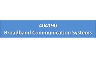
This paper discusses the impact of cloud attenuation on satellite network links in tropical regions like southwest Nigeria with high cloud cover percentages. The study focuses on improving satellite communication system design and operation by analyzing cloud effects and proposing modelling techniques for performance enhancement.

Uploaded on Oct 09, 2024 | 7 Views
Download Presentation

Please find below an Image/Link to download the presentation.
The content on the website is provided AS IS for your information and personal use only. It may not be sold, licensed, or shared on other websites without obtaining consent from the author.If you encounter any issues during the download, it is possible that the publisher has removed the file from their server.
You are allowed to download the files provided on this website for personal or commercial use, subject to the condition that they are used lawfully. All files are the property of their respective owners.
The content on the website is provided AS IS for your information and personal use only. It may not be sold, licensed, or shared on other websites without obtaining consent from the author.
E N D
Presentation Transcript
Cloud Attenuation Modelling for Satellite Network Links Performance Improvement O. M. Adewusi, T. V. Omotosho, M. L. Akinyemi, O. O. Ometan, S. A. Akinwunmi and A. A. Umar FoSC 2017 Department of Physics Lagos State University
OUTLINE OUTLINE Introduction Scenario Illustration Comparisons of The Foundation Cloud Models Station Cloud Cover Station Radiometric Data Acquisition and Analysis Cloud Attenuation Modelling Conclusion Future Work References
Introduction -1 Observations unavailability in most of the tropical region as southwest Nigeria is currently above the allowed 1% outage percentage and the tropical region cloud cover is averagely 70%, [2, 3]. The percentage of cloud attenuation in the total atmospheric attenuation effects is high, and moreover cloud is more persistent in the tropical region. show satellite services hydrometeors'
Figure 2: Cloud Types and Classification (Warren and Hans, 2002)
Satellite (E.g. ASTRA) Cloud Earth Satellite Antenna Concrete floor MModulato Modulator Demodulator High Power Amplifier Up Code Converter A/D Down Code Converter Low Noise Amplifier D/A Demodulator Indoor Unit Figure 3.0: Schematic Station Hydrometeor Attenuation Measurement Set up
Introduction - 2 Low clouds Stratus (St), Cumulus (C) Stratocumulus (Sc), Cumulonimbus (Cb), and Nimbostratus (Ns) have bases in the atmospheric boundary layer less than 2km above the earth surface; Middle or alto clouds Altostratus (As), Altocumulus (Ac) are clouds with bases 2 6km above the surface; High or cirro clouds cirrus (Ci), cirrocumulus (Cc) and cirrostratus (Cs) are clouds with bases between 6km above the surface and the tropopause [5] .
Introduction - 3 The effects of suspended water droplets (SWD) and suspended ice crystal (SIC) which constitute clouds are major concern in the design and successful operation of satellite communication system; at frequencies above 10GHz. Thus, for low-availability satellite services such as VSAT and USAT, at high frequencies, deep fades may occur, particularly in the tropics, due to higher probability of occurrence of cloud cover [2, 3].
Introduction - 4 The general objective of cloud models (Table 1) is to accurately estimate cloud liquid water amount for determination of amount of cloud attenuation along a satellite earth-space transmission path. Numerous cloud models have been independently developed over the last eight decades based on Rayleigh scattering and Mie absorption theories, using empirical data, [4].
Table 1:AComparative List of the Cloud Models. Model Name Gun and East (1954) Model Algorithm and Parameters Limitations = 0.4343 [6 / ( a )]Im [-( -1)/( +2)] 1 = Attenuation coefficient (dB / Km), a= density of water (g / cm-3) 1 = liquid water content of the cloud, = wavelength (cm) of incident signal Im = imaginary part of , = complex relative dielectric constant of water Staelin (1966) Valid for 10GHz to 37.5GHz = 1 [10^ (0.0122(291-T) - 6)] / ^2 ? = ?????????????????????? (?? 1) , 1 = liquid water content of the cloud (g/m3) T = temperature (K) , ? = wavelength (cm) of incident signal. Slobin (1982) Valid for 10GHz to 50GHz =4.343 1 [10^ (0.0122(291-T) -1)] 1.16 / ^2 ? = ?????????????????????? (??/??), 1 = liquid water content of the cloud T = temperature (K), ? = wavelength of incident signal
Table 1:AComparative List of the Cloud Models (2/3). Altshuler and Marr (1989) Valid between 15GHz to 100GHz. Assume 10 nominal cloud temperature Temperature limit: 10 10 frequency range 100GHz and above. ?.??? ??.?? ??.?+ ? ??? ? , for ?>8o A= ?.????+?.??????+ = {[(ae+ he) ^2 ae^2 Cos^2 ( )] ^ (1/2) aeSin ( )}, for 8 A = Attenuation (dB), ? = wavelength of incident signal, ? = surface absolute humidity , ? = elevation angle, ae = 8,497Km and he = (6.35 0.302 )Km o oC as b Liebe et al. (1989) = 1a? oC) + 273.15] 0C and ?=?????????????????????????? = 300/ [T ( = Attenuation coefficient (dB / Km), 1 = liquid water content of the cloud (g/m variable constants for different frequency ranges. 3), ? and ? are
Table 1:AComparative List of the Cloud Models (3/3). w (t, h) = wo exp(ct) [(h - hb) / hr ] Salonen (1990) WL (t, h) = W (t, h) Pw(t) ; W (t, h) = W (t, h) [1- Pw (t)] Where: Pw (t) = 1 + t/20, if -20 wo= 0.17 g/m 1, if 0 < t oC < t < 0 if t < -20 oC oC 0, -1 -3 and c = 0.04 Salonen and Uppala (1991) ITU-RP (2013) ?.???? ?"(?+??)????(?) ? ???? ?? ? = AL(P) = Slant Path Attenuation, P = Probability (%), ? = (2+? )?" ' and " are the real and imaginary parts of liquid water permitivity at O ??= ??? (dB/km) and ??= ? = ???/???? ??, ??? ? ?? L = total columnar content of cloud liquid water ? = Elevation angle; ??= specific attenuation coefficient. oC. 0.819? ?"(1+?2) dB/ km (g/m 3) -1
The Stations Cloud Cover The cloud cover of a station is a graphical relationship that shows the monthly variation of the percentage of cloud amount on the station s sky dome, thus daily total cloud amount need be accurately estimated by visual method or by an efficient cloud estimating instrument, and the monthly average total is computed through each year.
The Stations Cloud Cover -2 Cloud measurement method includes satellites cloud observations on one hand and visual measurement of cloud from the earth s surface stations on the other. On the visual measurement, each assessment view of the total amount of cloud entails determination of cloud amount in cloud layers between the cloud base and maximum vertical distance visible for each of the four sky quadrants during each of the fixed daily observation times.
The Stations Cloud Cover -3 Table 2 shows typical weekly record of the visual cloud data and Figure 4 shows the visual cloud cover result for. Table 2: Typical Visual Cloud Cover Weekly Record EAST (%) . . . . . . . NORTH (%) TCTP AVG. . . . . . . . 23.75 . . . . . . . 23.75 . . . . . . . 23.75 . . . . . . . 21.75 . . . . . . . 22 . . . . . . . A.M. P.M. A.M. P.M. AVG. TOTAL E S W N DATE 1-Aug 24 23.5 23.5 23 23.25 93.5 Ns ; Sc Ns ; Sc Ns ; Sc Ns ; Sc 2-Aug 24 23.5 24 24 24 95 Ns ; Ns, ScNs ; Ns, ScNs ; Ns, ScNs, Cu ; Ns, Sc 3-Aug 23.5 24 23.5 23.5 23.5 94.5 Ns ; Ns, Ns ; Ns, Ns ; Ns, Ns ; Ns, 4-Aug 23 20.5 23 22.5 22.75 90 Sc, Ns ;ScSc, ;Sc Sc, ;Sc, Ns Sc, ;Sc 5-Aug 21 23 21.5 23.5 22.5 88 St, ;Sc St, ;Sc St, Ac ; ScSt, Ac ; Sc
The Stations Cloud Cover -4 In the satellite observations segment of cloud cover determination for a station, radiance changes measured by satellites are interpreted using climatic models algorithms. For the case study station satellites 3-D cloud data are obtained from A- Train satellites, figure 5. Data from CLOUDSAT, CERES, TERA-AQUA-MODIS, CALIPSO, SRB and ISCCP satellites were downloaded and processed. Analyses of each set of satellite data were carried out and their output charts displayed in figure 6 are used for corroborating the surface visual cloud cover result.
Figure 6: OTA [CU] CLOUD COVER AND THE CORROBORATING SATELLITES OVER IT
Station Radiometric Data Acquisition In an observation station at least one radiometer will be required for radiometric data collection, and radiosonde data or satellite radiometric data will be needed for corroboration. In the Ota CU station case study, 9103 Spectrum Analyser is in use; fifty - three years radiosonde observations data was acquired, filtered and extracted to obtain each cloud layer s values for the required primary parameters pressure (hPa), temperature (K) and calculated geopotential height (m).
Station Radiometric Data Analysis Attenuation distribution and statistics for each of the eight listed cloud models were computed from the processed radiosonde data. The station logged spectrum analyser data (SPAD) were extracted and analysed under two conditions - rainy and non-rainy days, using the climatological device s monthly data for each year. Then all the processed data for three years were integrated and the integrated data cumulative distribution curve obtained.
Station Radiometric Data Analysis - 2 Each distribution curve is a result of raw data processing using electronic spread sheet programming to implement several layers of required station conditions geographic, climatic and spectra conditions. The resulting cloud attenuation cumulative distribution curves at 12.5 GHz for each of the existing cloud models and that for the spectrum analyser compared in figure 9. such as data (SPAD) were
Figure 9: SPAD and Cloud Models Distribution Curves at 12.5 GHz
Cloud Attenuation Modelling The SPAD integrated attenuation cumulative distribution curve approximates a straight line of slope - 0.31011 and intercepts 3.089 dB, which appear as a resultant constructive interference of some pairs of periodic functions of comparable amplitudes. A possible general mathematical representation of these observations is equation (1): Ac(WL, , t, f) = f(x) = acos(x) + bsin(x) = Acos(x ) (1)
Cloud Attenuation Modelling - 2 where A = (a2 + b2)1/2and = tan-1(b/a) in the range 0 < < /2; considering the variables of the cloud attenuation (Ac) - cloud liquid water content (WL) of each cloud layer series (CLS) and their temperature (t); angle of elevation ( ) and frequency (f) of propagating radio signals; x is considered to be cloud layer specific attenuation coefficient (KL) defined in the International Telecommunication Union Recommendation (ITU-R) P.840 4, corresponding to the frequency function g(f) in the Salonen Uppala procedure [6].
Cloud Attenuation Modelling - 3 Considering the relatively gentle slope of the SPAD line, the range of x should be 0 to rather than 0 to /2, and using the straight line analogue, a = - 0.31011, b = 3.089 dB, as directly measured from the graph; A = 3.08915 and = - 1.560796 by computation; hence the equation (1) becomes: Ac = 3.08915WLCOS ((0.5KL) + 1.560796) 0 KL (2)
Cloud Attenuation Modelling - 4 Situations of constants and constant variable parameters of the equation having more than one possible form or value are resolved by generating the distribution corresponding to each of the most probable options. The option whose chart is closest to that of the station measured data distribution (SPAD) is taken. and chart
Cloud Attenuation Modelling - 5 Then the proposed model i.e. equation (2) is tested by comparing its performance with those of the standard cloud models at the station as shown in Figures 10 14.
Figure 10: Cloud Attenuation Models Distribution Curves at 12.5 GHz
FIGURE 11: OTA CU CLOUD MODEL Vs FOUNDATION MODELS AT 12 GHz
FIGURE 12: OTA CU CLOUD MODEL Vs FOUNDATION MODELS AT 14 GHz
FIGURE 13: OTA CU CLOUD MODEL Vs FOUNDATION MODELS AT 20 GHz
FIGURE 14: OTA CU CLOUD MODEL Vs FOUNDATION MODELS AT 30 GHz
Cloud Attenuation Modelling - 6 Hence equation (2) represents the cloud attenuation model for the station having shown considerable agreement with the foundation models at various frequencies. geometric pattern
Future Work Radiometric measurements, cloud visual data and climatological data acquisition need to start and continue in every climatic zone of Nigeria, i.e. about every state of the federation, particularly in high tele-density areas as Lagos state, to enable development of relevant hydrometeors models and corresponding cloud attenuation statistics. However, a single global satellite based climatic model is desirable, where modular algorithm would be used to integrate the various climatic zones models.
References [1] Das S, Chakraborty S and Maitra A, (2013): Radiometric cloud attenuation at a tropical location in India; Journal of Atmospheric and Solar-Terrestrial Physics, (105-106): 97-100. Eva R I, Gustavo A S, Jose M R, and Pedro G P, (2015): Atmospheric Attenuation in Wireless Communication Systems at Millimeter and THz Frequencies; IEE Antenna and Propagation Magazine, 57 (1): 48- Omotosho T V, Mandeep J S and Mardina A, (2013): Cloud Attenuation Studies of the Six Major Climatic Zones of Africa for Ka Satellite System Design; Annals of Geophysics; 56 (6): 1-2. Gerace G C and Smith E K, (1990): A Comparison of Cloud Models; Antennas and Propagation Magazine. Warren, S. G. and Hahn, C. J. (2002): Climatology; Encyclopedia of Atmospheric Sciences, Academic Press. Salonen, E. and Uppala, S. (1991): New prediction method of cloud attenuation; Electron, Lett 27, measurements of [2] 61. [3] and V [4] IEEE [5] [6] 1106-1108.


.")