Efficient Parameter-free Clustering Using First Neighbor Relations
Clustering is a fundamental pre-Deep Learning Machine Learning method for grouping similar data points. This paper introduces an innovative parameter-free clustering algorithm that eliminates the need for human-assigned parameters, such as the target number of clusters (K). By leveraging first neighbor relations, this approach streamlines the clustering process without requiring additional information beyond the data itself. The technique enhances efficiency and removes the burden of parameter selection in clustering tasks. Additionally, it incorporates optimization strategies for faster computation of pairwise distances, improving overall clustering performance.

Uploaded on Sep 15, 2024 | 1 Views
Download Presentation

Please find below an Image/Link to download the presentation.
The content on the website is provided AS IS for your information and personal use only. It may not be sold, licensed, or shared on other websites without obtaining consent from the author.If you encounter any issues during the download, it is possible that the publisher has removed the file from their server.
You are allowed to download the files provided on this website for personal or commercial use, subject to the condition that they are used lawfully. All files are the property of their respective owners.
The content on the website is provided AS IS for your information and personal use only. It may not be sold, licensed, or shared on other websites without obtaining consent from the author.
E N D
Presentation Transcript
Efficient Parameter-free Clustering Using First Neighbor Relations Paper By: M. Saquib Sarfraz, Vivek Sharma, Rainer Stiefelhagen Presented By: Craig Kenney
Clustering Clustering is one of the core pre-Deep Learning Machine Learning methods. It is unsupervised learning, and it aims to group similar data points together into groups. There are three categories of clustering methods: Centroid (K-Means), Agglomerative, and Graph (Spectral Methods).
Clustering Methods K-means K-means clustering begins with K clusters, either partitioned randomly, based on random points as center, or other, more complex methods. Then, the clusters are iteratively updated by calculating the center of each cluster, and assigning points to the cluster whose center they are closest to each step. The algorithm is finished when iteration no longer changes the cluster assignments.
Clustering Methods - Agglomerative Agglomerative clustering begins by treating every single data point as its own cluster, and then repeatedly merging the clusters which are closest to each other, until the target number of clusters is reached. This can be done in a variety of ways, depending on how distance is calculated for example: using the center of each cluster, using the minimum or maximum distances between points in the two clusters, and so on.
Parameter-free The existing methods of clustering all have something in common they need to have parameters assigned by an expert. Most significantly, K, the target number of clusters in the final clustering. This requires some determination to be made about what types of clustering would be useful based on the data alone, which could be error-prone, or lead to running the clustering algorithm many times to find the set of parameters that creates the most useful result. This paper s clustering algorithm removes this element entirely, and is capable of clustering with no extra information beyond the data itself.
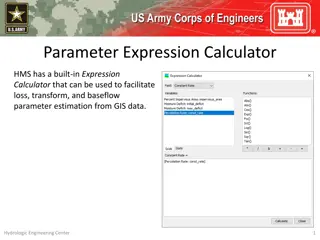
Background - Approximation M. Muja and D. G. Lowe. Scalable nearest neighbor algorithms for high dimensional data. PAMI, 2014. This paper is the source of a fairly important optimization used in the clustering algorithm. Usually, a clustering algorithm will need to calculate pairwise distances for all points when determining distances, but using the randomized k-d algorithm from this paper they can find the first nearest neighbor much faster.
Technique Concept The primary point that the paper makes, is that typical clustering methods work by interpreting direct distances between data points, which can get less than useful at higher dimensions. They instead want to rely on semantic links, rather than direct distances. In this case, the semantic link their clustering algorithm focuses on is the very first neighbor of each point the single other point that it is closest to.
The Clustering Algorithm They first construct an adjacency matrix using the above equation, with i and j representing any two data points, and and being their respective first neighbors. So, in the graph created by this adjacency matrix, data points will be connected if they either are related as first neighbors, or if they share the same first neighbor. Finally, the clusters are the connected components of the created graph.
Simple Example First Neighbors To get a better idea of how the clustering algorithm works, there is a simple example using 8 planets and the moon. The data is taken from NASA s planetary fact sheet, using the first 15 data attributes, creating the table of first neighbors we can see here. Distance calculated is pairwise Euclidean distance.
Simple Example Adjacency Matrix Then, using the simple formula from before, we can create the adjacency matrix from that set of first neighbors.
Simple Example - Graph And if we take that adjacency matrix and create a graph, we can easily see how that graph has been broken into three connected segments, these are our clusters. These clusters match a grouping made by astronomers into rocky planets(Venus, Earth, Mars, Moon, Mercury), gas planets(Saturn, Jupiter), and ice giants(Neptune, Uranus).
The Clustering Algorithm In Practice In practice, however, the algorithm is not used in its simplest form. Instead of simply running the algorithm once, it is run recursively, using the clusters from the first partition as data points in the next partition, in a manner similar to agglomerative clustering. This is repeated until all clusters have been merged into one, and then the total set of all partitions is the output, a clustering hierarchy. They call their algorithm FINCH, for the First Integer Neighbor it uses and the Clustering Hierarchy it produces.
Experimental Setup - Data Mice Protein expression levels of 77 proteins. Reuters 800000 news articles, of which they use a sampled subset of 10000. (TF- IDF features are 2000 dimensions.) STL-10 - image recognition dataset, 10 classes with 1300 examples each. BBTs01 and BFs05 facial recognition/clustering on episodes of tv shows. MNIST three variants of the MNIST handwritten digits dataset, MNIST_10k, MNIST_70k, and MNIST_8M. For STL-10, BBTs01, and BFs05 they rely on features from a CNN, and for MNIST they test separately on both features from a CNN and the pixels of the image.
Results Large-Scale Datasets When moving to larger scale datasets, very few of the other clustering algorithms were capable of scaling to meet the size of the datasets.
Results - Speed They attribute FINCH s speed advantage to the simplicity of the first neighbor calculation, which can be done using fast approximation methods, the one they use here is kd-tree.
Results Convergence Rate The cluster count does not ever hit exactly 1 as for these tests they made use of a ground truth clustering and stopped once that had been matched.
Results Deep Clustering Deep Clustering is a somewhat recent idea to use clustering as part of the learning system of a CNN. They use FINCH here to generate clusters that they then use as labels in training their neural network. They train in steps, using the initial FINCH labels, then re-clustering to update the labels every 20 epochs, for a total of 60-100 epochs. For this test they use 2 hidden layers with 512 neurons each, batch size 256, and initial learning rate 0.01.
Conclusions They have managed to create a new form of clustering that requires no hyperparameters from the user, and can run much faster through approximation rather than needing to calculate the full pairwise distance matrix.
Sources and References Original Paper: M. S. Sarfraz, V. Sharma, R. Stiefelhagen, Efficient Parameter-free Clustering Using First Neighbor Relations (arXiv:1902.11266) Background Information: M. Caron, P. Bojanowski, A. Joulin, and M.Douze, Deep Clustering for Unsupervised Learning of Visual Features (arXiv:1807.05520) M. Muja and D. G. Lowe. Scalable nearest neighbor algorithms for high dimensional data. PAMI, 2014.