Distances to Core-Collapse Supernovae & Methods of Measurement
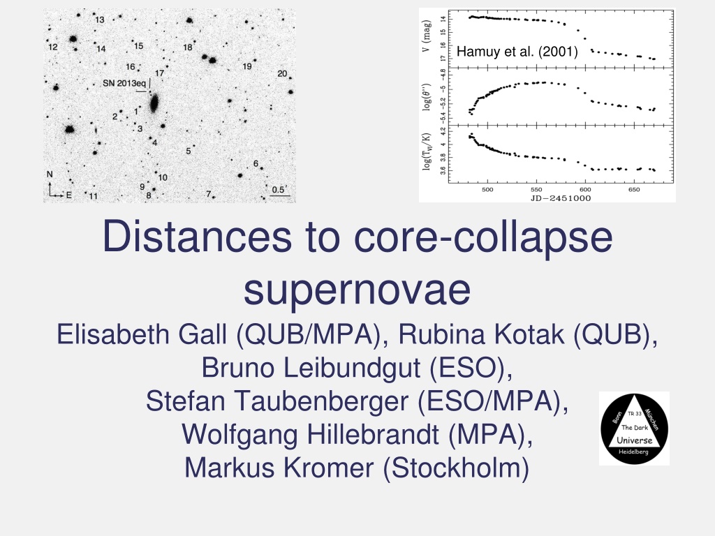

Distances to core-collapse
supernovae
Elisabeth Gall (QUB/MPA), Rubina Kotak (QUB),
Bruno Leibundgut (ESO),
Stefan Taubenberger (ESO/MPA),
Wolfgang Hillebrandt (MPA),
Markus Kromer (Stockholm)
Extragalactic Distances
•
Many different methods
–
Galaxies
•
Mostly statistical
•
Secular evolution, e.g. mergers
•
Baryonic acoustic oscillations
–
Supernovae
•
Excellent (individual) distance indicators
•
Three main methods
–
(Standard) luminosity, aka ’standard candle’
–
Expanding photosphere method
–
Angular size of a known feature
Physical parameters of core
collapse SNe
•
Light curve shape and the velocity
evolution can give an indication of the
total explosion energy, the mass and
the initial radius of the explosion
Observables:
•
length of plateau phase
Δ
t
•
luminosity of the plateau L
V
•
velocity of the ejecta v
ph
•
E
Δ
t
4
·v
ph
5
·L
-1
•
M
Δ
t
4
·v
ph
3
·L
-1
•
R
Δ
t
-2
·v
ph
-4
·L
2
Expanding Photosphere
Method
•
Modification of Baade-Wesselink
method for variable stars
•
Assumes
–
Sharp photosphere
thermal equilibrium
–
Spherical symmetry
radial velocity
–
Free expansion
Photosphere Expansion
•
Measured from absorption lines
–
formed close to the photosphere
•
not hydrogen lines
Fe II
–
remove redshift (from galaxy spectrum)
•
Colour
–
K-corrections
(redshift)
Photosphere Expansion
Expanding Photosphere Method
Expanding Photosphere Method
•
Multiple filters
•
Influence of known date of explosion
Expanding Photosphere Method
Expanding Photosphere Method
•
Principle difficulties
–
Explosion geometry/spherical symmetry
–
Uniform dilution factors?
•
Develop tailored spectra for each supernova
Spectral-fitting Expanding Atmosphere
Method (SEAM)
–
Absorption
•
Observational difficulties
–
Needs multiple epochs
–
Spectroscopy to detect faint lines
–
Accurate photometry
Hubble Diagram
•
Independent of distance ladder
Standardizable Candle
Method
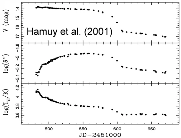
Introduced by Hamuy &
Pinto (2002)
–
Normalised luminosity
during the plateau
phase of SNe IIP
–
Normally at 50 days
after explosion
Used widely for SNe IIP
–
Nugent et al. 2006
–
Poznanski et al. 2009
–
Olivares et al. 2010
–
Maguire et al. 2010
–
Polshaw et al. 2015
Standardizable Candle
Method
•
Straightforward simple method
–
Only few observations required
•
Issues
–
Need to know explosion time
•
Often not too obvious from observational data
–
Measurement during a ’faint’ epoch
•
Plateau and not maximum
–
Spectroscopy often difficult
•
Faint phase and faint lines
•
Attempts to use prominent hydrogen lines
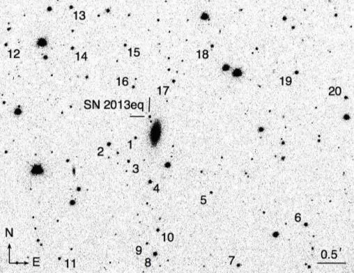
Distance to SN 2013eq
(z=0.041)
•
Use EPM and CSM to measure
distance to same supernova
•
EPM provides explosion date to be
used by CSM
Gall et al. 2016
Testing GR
This study explores the distances to core-collapse supernovae using various methods such as the expanding photosphere method and physical parameters analysis. The research delves into extragalactic distances, the photosphere expansion, and modification of existing methods to determine accurate distances in the context of stellar evolution.

Download Presentation

Please find below an Image/Link to download the presentation.
The content on the website is provided AS IS for your information and personal use only. It may not be sold, licensed, or shared on other websites without obtaining consent from the author. Download presentation by click this link. If you encounter any issues during the download, it is possible that the publisher has removed the file from their server.
E N D
Presentation Transcript
Hamuy et al. (2001) Distances to core-collapse supernovae Elisabeth Gall (QUB/MPA), Rubina Kotak (QUB), Bruno Leibundgut (ESO), Stefan Taubenberger (ESO/MPA), Wolfgang Hillebrandt (MPA), Markus Kromer (Stockholm)
Extragalactic Distances Many different methods Galaxies Mostly statistical Secular evolution, e.g. mergers Baryonic acoustic oscillations Supernovae Excellent (individual) distance indicators Three main methods (Standard) luminosity, aka standard candle Expanding photosphere method Angular size of a known feature
Physical parameters of core collapse SNe Light curve shape and the velocity evolution can give an indication of the total explosion energy, the mass and the initial radius of the explosion Observables: length of plateau phase t luminosity of the plateau LV velocity of the ejecta vph E t4 vph5 L-1 M t4 vph3 L-1 R t-2 vph-4 L2
Expanding Photosphere Method Modification of Baade-Wesselink method for variable stars Assumes Sharp photosphere thermal equilibrium Spherical symmetry radial velocity Free expansion Kirshner & Kwan 1974
Photosphere Expansion Measured from absorption lines formed close to the photosphere not hydrogen lines Fe II remove redshift (from galaxy spectrum) Colour K-corrections (redshift) 0.6 1.0 observedspectrum rest framespectrum Gall 2016 r r r 0.8 i i i g g g Normalizedflux u u u z z z 0.4 0.2 0.0 9000 3000 4000 5000 6000 Wavelengthin A 7000 8000 10000 Figure 2.6: Observed (black) and rest frame (cyan) spectrum of SN 2013eq (z = 0.041 0.001) obtained with theOSIRISmounted on theGTC on October 6th, 2013, overlaidwiththeSDSSu g r i z filter transmissioncurves. theproblem arising for broad-band photometric measurementsdueto thisshift in the spectrum. For example, whilein theobserved frametheprominent H emission con- tributesonly very littletowardsther magnitude, in theSN frametheH emission is almost entirely encompassed by thefilter. Consequently, observed magnitudesdo not necessarily reflect the true SN brightness. The transformation between the observed apparent magnitude,mx, inafilter x, totherest frameabsolutemagnitude, My, inadif- ferent filter yrequirestheaidof K-corrections(Oke& Sandage1968; Kimet al. 1996; Hogget al. 2002): My= mx Ax Kxy, (2.2) where isthedistancemodulus, Axistheforegroundreddeningextinctiontoward the sourceintheobservedfilter xand KxyistheK-correction fromobservedfilter xtorest framefilter y. It isdefinedas(followingtheformulationof Hogget al. 2002): , gy L ( )Sy( ) d L ( gx 1+z)Sx( ) d ( )Sx( ) d ( )Sy( ) d 1 Kxy= 2.5log (2.3) 1+ z wherezistheredshift of theSN, / L ( ) istheluminosityof thesourceat thewavelength ,Sx/y( ) arethefilter responses of the x and y filters per unit wavelength and gx/y wavelengthfor astandardsourceinthexandyfilters. arethewavelengthsin therest/observed frame, ( ) are the flux densities per unit K-correctionswerecomputedby usingtheacquired spectraof arespectiveSN and thesnakecode(SuperNovaAlgorithmfor K-correctionEvaluation)withintheS3pack- 29
Photosphere Expansion luminosity radius temperature Hamuy et al. (2001) Elmhamdi et al. (2003)
Expanding Photosphere Method 2?? ? ; ? = ? ? ?0 + ?0; ??=? R from radial velocity Requires lines formed close to the photosphere D from the surface brightness of the black body Deviation from black body due to line opacities Encompassed in the dilution factor ?2 ? =? ?? ?= ?(? ?0) ??
A&A proofs: manuscript no. WholeSample_paper 0.25 0.25 B: DL= 325 200Mpc V: DL= 282 161Mpc I: DL= 319 113Mpc B: DL= 347 200Mpc V: DL= 302 161Mpc I: DL= 341 115Mpc 0.20 0.20 0.15 0.15 Mpc Mpc d d = = 2v 2v 0.10 0.10 Expanding Photosphere Method 0.05 0.05 0.00 0.00 PS1-13wr PS1-13wr Multiple filters Influence of known date of explosion 0 20 40 0 20 40 40 20 Epoch relativetodiscovery (rest frame) 40 20 Epoch relativetodiscovery (rest frame) Fig.C.3: Distancefit for PS1-13wr using BVIasgiveninHamuy et al.(2001) (left panel) andDessart & Hillier (2005) (right panel). Thediamond markersdenotevaluesof through which thefit ismade. E.E.E. Gall et al.: AnupdatedTypeII supernovaHubblediagram 0.14 0.16 0.16 0.14 B: DL= 357 43Mpc V: DL= 349 34Mpc I: DL= 366 29Mpc B: DL= 409 49Mpc V: DL= 399 39Mpc I: DL= 419 33Mpc I: DL= 989 409Mpc B: DL= 1149 887Mpc V: DL= 624 214Mpc B: DL= 1147 953Mpc V: DL= 649 201Mpc I: DL= 1005 356Mpc 0.14 0.14 0.12 0.12 0.12 0.12 0.10 0.10 0.10 0.10 0.08 0.08 Mpc Mpc Mpc Mpc d d d d 0.08 0.08 = = 2v 2v 2v 0.06 0.06 0.06 = = 2v 0.06 0.04 0.04 0.04 0.04 0.02 0.02 0.02 0.02 0.00 0.00 0.00 PS1-12bku PS1-12bku PS1-14vk 0.00 PS1-14vk 0 10 Epoch relativetodiscovery (rest frame) 20 30 40 0 10 Epoch relativetodiscovery (rest frame) Epoch relativetodiscovery (rest frame) 20 30 40 0 20 40 0 20 40 100 80 60 40 20 100 80 60 Epoch relativeto discovery (rest frame) 40 20 Gall et al., in prep. Fig. C.4: Distance fit for PS1-12bku using BVIas given in Hamuy et al. (2001) (left panel) and Dessart & Hillier (2005) (right panel). Thediamond markersdenotevaluesof throughwhich thefit ismade. Hillier (2005) (right panel). Thediamond markersdenotevaluesof through whichthefit ismade. Fig. 4: Distance fit for PS1-14vk using all available epochs and BVIas given in Hamuy et al. (2001) (left panel) and Dessart & 0.16 0.16 B: DL= 474 54Mpc V: DL= 440 47Mpc I: DL= 463 47Mpc B: DL= 505 58Mpc V: DL= 469 50Mpc I: DL= 494 50Mpc I: DL= 534 210Mpc 0.12 0.12 B: DL= 532 738Mpc V: DL= 375 142Mpc B: DL= 564 570Mpc V: DL= 403 142Mpc I: DL= 567 203Mpc 0.14 0.14 0.10 0.10 0.12 0.12 0.08 0.08 0.10 0.10 Mpc Mpc Mpc d d Mpc 0.06 0.06 0.08 d d 0.08 = = = 2v 2v = 2v 2v 0.04 0.06 0.06 0.04 0.04 0.04 0.02 0.02 0.02 0.02 0.00 0.00 0.00 PS1-13abg PS1-13abg PS1-14vk 0.00 PS1-14vk 10 0 10 20 30 40 10 0 10 20 30 20 40 Epoch relativetodiscovery (rest frame) Epoch relativetodiscovery (rest frame) 20 Epoch relativetodiscovery (rest frame) 40 0 40 40 20 Epoch relativeto discovery (rest frame) 0 20 40 Fig. C.5: Distance fit for PS1-13abg using BVIas given in Hamuy et al. (2001) (left panel) and Dessart & Hillier (2005) (right panel). Thediamond markersdenotevaluesof throughwhich thefit ismade. Fig. 5: Distancefit for PS1-14vk usingonly thoseepochsthat follow alinear relation and BVIasgiven inHamuy et al. (2001) (left panel) and Dessart & Hillier (2005) (right panel). Thediamond markersdenotevaluesof through which thefit ismade. ously been observed (e.g. Hamuy et al. 2001; Jones et al. 2009). For some SNe the photometry provides independent esti- mates of the time of explosion. In theses cases we use the observed explosion epoch as an additional data point in the fit and are able to significantly reduce the error in the distancedetermination. In Section 3.4.2 wederived an epoch dependent vH /vFe5169 ratio, which after about 30 days begins to diverge signifi- cantly for the individual SNe. In those cases where we ap- ply thisratio, wethereforeonly includedataup to 30 days from explosion. Joneset al. (2009) arguethat after around 40 daysfrom ex- plosion the linearity of the /v versus t relation in Type II- P SNe deteriorates. Considering the scarcity of data points for our SNe, we use data up to 60 days from explosion for the distance fits, whenever viable. For most SNe in our sample the -t relation seems to be linear also in this ex- tended regime. The exception is the PS1-14vk; a Type II-L SN.A comparisonbetweenFigures4and5clearly illustrates abreakdown in thelinearity of the -t relation in theinter- val between +33 and +49 days. When performing a -t fit beyondthelinear regimethedistancesareoverestimatedsig- nificantly and theestimated epoch of explosion isconsider- ably earlier than when using only thelinear regime. In light of PS1-14vk being a Type II-L SN, this raises the question whether the -t relation isgenerally valid for ashorter pe- riodof timein SNeII-L compared to SNeII-P . Our errors on the distances (averaged over the BVI filters) spanawiderangebetween 3%and 54%, essentially de- pendingonthequality of theavailabledatafor each SN. E.g. astrongconstraint ontheepochof explosionreducestheun- certainty of the distance fit significantly. Our final as well asintermediateerrorsaccount for theuncertaintiesfrom the photometry, the SN redshift, the K-corrections, the photo- spheric velocitiesand for theSNe2013eq andPS1-13wr thedust extinctionin thehost galaxy. Articlenumber, page36 of 37page.37 Our intermediate results are presented in Table B.3 in the appendix and a summary in Table 4. We have taken great care to proceed with all SNe in the same manner as far as possi- ble. Nonetheless, a case-by-case evaluation cannot be avoided entirely. In the following we outline the particularities for each individual SN. Articlenumber, page9of 37page.37
Expanding Photosphere Method Measures an angular size distance Not important in the local universe Interesting for cosmological applications Mostly for H0 Cosmology Include time dilation Metric theories of gravity imply ??= 1 + ?2??
Expanding Photosphere Method Principle difficulties Explosion geometry/spherical symmetry Uniform dilution factors? Develop tailored spectra for each supernova Spectral-fitting Expanding Atmosphere Method (SEAM) Absorption Observational difficulties Needs multiple epochs Spectroscopy to detect faint lines Accurate photometry
E.E.E. Gall et al.: AnupdatedTypeII supernovaHubblediagram Table5: SCM quantitiesand distances Estimate of t0via EPM H01 EPM D05 G15 EPM H01 EPM D05 EPM H01 EPM D05 PS1 PS1 PS1 PS1 EPM H01 t0 V mag I 50 mag v50 Estimateof velocity via DL Mpc 180 36 176 34 385 67 438 115 430 114 394 136 396 133 286 31 730 107 832 194 684 87 1348 470 1368 487 SN 50 kms 1 5427 798 5228 758 5616 655 4458 963 4368 959 5228 818 5093 816 4258 291 4672 438 4093 473 4363 256 5814 1175 5913 1237 mjd mag 56382.3+9.7 56386.1+5.9 56593.4 0.7 56330.5 12.5 56332.2 12.1 56717.0 10.1 56719.6 9.7 56160.9 0.4 56375.4 5.0 56408.0 1.5 56420.0 0.1 56401.3 7.9 56400.0 8.6 19.08 0.10 19.12 0.10 20.61 0.10 21.38 0.06 21.39 0.06 20.95 0.29 21.02 0.27 20.70 0.07 22.27 0.08 23.06 0.22 22.51 0.06 23.39 0.26 23.39 0.26 18.56 0.08 18.59 0.08 20.00 0.09 20.49 0.07 20.49 0.07 20.63 0.24 20.68 0.23 20.18 0.06 21.12 0.09 22.38 0.12 21.92 0.11 23.18 0.20 23.19 0.20 36.28 0.43 36.22 0.42 37.93 0.38 38.21 0.57 38.17 0.58 37.98 0.75 37.99 0.73 37.28 0.23 39.32 0.32 39.60 0.51 39.18 0.28 40.65 0.76 40.68 0.77 SN 2013ca Feii 5169 10.1 9.4 LSQ13cuw H PS1-13wr Feii 5169 PS1-14vk PS1-12bku PS1-13abg PS1-13baf PS1-13bmf Feii 5169 Feii 5169 Feii 5169 H Feii 5169 Hubble Diagram PS1-13bni EPM D05 H Independent of distance ladder K-corrected magnitudesintheJohnson-CousinsFilter System. H01: Hamuy et al. (2001); D05: Dessart & Hillier (2005). 42 42 EPM Gall et al., in prep SCM PS1-13bmf PS1-13bmf 40 1000 40 1000 PS1-14vk PS1-14vk LSQ13cuw LSQ13cuw 38 38 36 36 DL[Mpc] DL[Mpc] 100 100 34 34 32 32 Thiswork: D05 H Phot H D05 Fe Phot Fe P09 P09culled O10 A10 Thiswork: E96 J09 B14 D05 Fe D05 H 30 10 30 10 H0= 70 5kms 1Mpc 1 m= 0.3, = 0.7 H0= 70 5kms 1Mpc 1 m= 0.3, = 0.7 28 28 0.001 0.002 0.005 0.01 0.02 z 0.05 0.1 0.2 0.3 0.001 0.002 0.005 0.01 0.02 z 0.05 0.1 0.2 0.3 Fig. 7: SN II Hubble diagram using the distances determined via the EPM (left panel) and the SCM (right panel). EPM Hubble diagram (left): the distances derived for our sample (circles) use the dilution factors published by Dessart & Hillier (2005). The different colours (red/blue) denote the line that was used to estimate the photospheric velocities of the particular SN (Feii 5169 or H ). Wealso included EPM measurements from the samples of Eastman et al. (1996, E96), Jones et al. (2009, J09) and Bose & Kumar (2014, B14). The solid line corresponds to a CDM cosmology with H0= 70kms 1Mpc 1, m= 0.3 and = 0.7, and thedotted linesto therangecovered by an uncertainty of 5kms 1Mpc 1. SCM Hubblediagram (right): circlemarkersdepict the SCM distances derived for our sample using the explosion epochs previously derived via the EPM and applying the dilution factorspublished in Dessart & Hillier (2005). Thestar shaped markersdepict thoseSNefor which an independent estimateof the explosiontimewasavailableviaphotometry. Thecoloursarecodedinthesameway asfor theEPM Hubblediagram. Similarly, the solid and dotted linesportray thesamerelation between redshift and distancemodulusasin theleft panel. Wealso included SCM measurements from thesamples of Poznanski et al. (2009, P09, which includesall objectsfrom theNugent et al. (2006) sample), Olivareset al. (2010, O10) and D Andreaet al. (2010, A10). Weseparated theobjects culled by Poznanski et al. (2009) from the rest of thesampleby usingadifferent symbol. ThethreeTypeII-L SNeLSQ13cuw,PS1-14vk andPS1-13bmf areidentifiedinboth theEPM andtheSCM Hubblediagram. (1996, Table6), Joneset al. (2009, Table5) and Bose& Kumar (2014, Table 3) in the EPM Hubble diagram (see left panel of Figure 7). These values were adopted as they are, without any correction for potential systematic differences. In the cases of Jones et al. (2009) and Bose & Kumar (2014) we selected the distances given using theDessart & Hillier (2005) dilution fac- tors. Inaddition, Bose& Kumar (2014) givealternateresultsfor theSNe 2004et, 2005cs, and 2012aw, for which constraints for theexplosion epoch areavailable. Wechosethesevaluesrather than the less constrained distance measurements in these three cases. Notethat theJoneset al. (2009) samplehasSN 1992bain common with theEastman et al. (1996) sampleand SN 1999gi common with theBose& Kumar (2014) sample. ExploringtheEPM Hubblediagram,itisimmediately appar- ent that our measured distances follow the slope of the Hubble line,despitetherather poor quality of thedataavailablefor some of our SNe. 3.8.2. SCM Hubble diagram The SCM Hubble diagram shows the SCM distances derived for our sample alongside SCM measurements from the sam- Articlenumber, page13 of 37page.37
Standardizable Candle Method Introduced by Hamuy & Pinto (2002) Normalised luminosity during the plateau phase of SNe IIP Normally at 50 days after explosion Used widely for SNe IIP Nugent et al. 2006 Poznanski et al. 2009 Olivares et al. 2010 Maguire et al. 2010 Polshaw et al. 2015 Hamuy & Pinto 2002
Standardizable Candle Method Straightforward simple method Only few observations required Issues Need to know explosion time Often not too obvious from observational data Measurement during a faint epoch Plateau and not maximum Spectroscopy often difficult Faint phase and faint lines Attempts to use prominent hydrogen lines
A&A 592, A129(2016) Table2. EPM quantitiesfor SN 2013eq. Epoch rest frame Averagedv kms 1 Dilution factor BVI reference 0.41 0.53 0.43 0.59 0.75 0.92 Date MJD V 1012 4.8 1.5 4.2 1.3 6.1 1.3 5.3 1.1 10.5 1.4 9.5 1.2 B 1012 4.9 1.8 4.4 1.6 6.1 1.5 5.3 1.3 8.8 1.5 8.0 1.4 I 1012 5.3 1.2 4.7 1.1 6.1 0.9 5.3 0.8 8.8 0.8 8.0 0.7 H01 D05 H01 D05 H01 D05 2013-08-15 56519.96 +15.44 6835 244 2013-08-25 56529.96 +25.05 5722 202 2013-10-06 56571.90 +65.34 3600 104 Notes.( )Rest frameepochs(assuming aredshift of 0.041) with respect to thefirst detection on 56503.882 (MJD). H01: Hamuy et al. (2001); D05: Dessart & Hillier (2005). SeealsoFig. 4. Distance to SN 2013eq (z=0.041) Use EPM and CSM to measure distance to same supernova Fig. 4. Distancefit for SN 2013eq using BVIasgiven in Hamuy et al. (2001; left panel) and Dessart & Hillier (2005; right panel). Thediamond markersdenotevaluesof through whichthefit ismade; circlemarkersdepict theresulting epochof explosion. EPM provides explosion date to be used by CSM Table3. EPM distanceandexplosion timefor SN 2013eq. Gall et al. 2016 t3 0 t? 0 Averaget? days Dilution factor DL Mpc 163 45 125 22 165 23 177 48 136 23 180 25 Averaged DL Mpc Filter 0 days 5.8 10.5 0.5 5.4 7.1 6.0 4.7 9.8 1.3 5.1 5.9 5.6 MJD B V I B V I H01 151 18 4.1 4.4 56499.6 4.6 D05 164 20 3.1 4.1 56500.7 4.3 Notes.( )Rest framedaysbeforediscovery on56503.882 (MJD). H01: Hamuy et al. (2001); D05: Dessart & Hillier (2005). SeealsoFig. 4. determining theexpansion velocity at 50 days, although theer- ror intheFeii 5169velocitiesandtheintrinsicerror inEq.(12) alsocontributetothetotal error. 4.5. Comparison of EPM and SCM distances An inspection of Table 3 reveals that the two EPM luminosity distances derived using the dilution factors from Hamuy et al. (2001) andDessart & Hillier (2005) giveconsistent values. This is no surprise, bearing in mind that the dilution factors from Hamuy & Pinto (2002) andDessart & Hillier (2005) applied for SN 2013eq di er by only 18 27% (seeTable2). Similarly, the resulting explosion epochsarealsoconsistent witheachother. Likewise, the SCM distances calculated utilizing the times of explosion foundviaEPM andthedilution factorsfromeither Hamuy & Pinto (2002) or Dessart & Hillier (2005,seeTable4), as well as by adopting the average SN II-P rise time as given by Gall et al. (2015), areconsistent not only with each other but also withtheEPM results. The uncertainty in the redshift plays an almost negligible role. For completenesswedidhowever propagateitserror when accounting for time dilation. Note that Hamuy & Pinto (2002) find peculiar motions in nearby galaxies (cz < 3000kms 1) contributesignificantly totheoverall scatter intheir Hubbledia- gram; however thisisnot arelevant issuefor SN 2013eq. Thefinal uncertainties in thedistance modulusand thedis- tancearepropagatedfromtheerrorsinMI50,v50,Feiiand(V I)50. Thederiveddistancemoduli andluminosity distancesaswell as theintermediateresultsaregiveninTable4. A129, page8of 12
Testing GR A&A proofs: manuscript no. WholeSample_paper SN. The derived explosion epoch isthen used as abase for the second iteration, and the spectral epochs as well as vH /vFe5169 ratiosareadjusted accordingly. Werepeat thisprocessuntil the explosion timeconverges. Gall et al., in prep 2.0 3.6. SCM distances 1.5 / DSCM PS1-14vk In order to apply the SCM the SN magnitudes have to be con- vertedtotherest frame. WeusetheV- and I-band K-corrections that werealready evaluatedfor theEPM.Thesearetheninterpo- lated to 50d after explosion and used to correct theinterpolated 50d photometry. Theexpansionvelocity isdeterminedusingtherelationpub- lished by Nugent et al. (2006, Equation 2): L DEPM L PS1-13bmf 1.0 DEPM L = DSCM L 0.5 0.464 0.017 t 50 Fe H LSQ13cuw v50= v(t ) , (4) 500 1000 1500 [Mpc] 2000 2500 DEPM L wherev(t ) istheFeii 5169 velocity at timet after explosion (rest frame).For theSNewherewecouldnot identify Feii 5169 featureintheir spectrawefirst appliedeither thevH - vFe5169or thevH - vFe5169relationandthenutilizedthederivedFeii 5169 velocitiestoestimatetheexpansionvelocity at day 50. Thispro- cedurewasrepeated twicefor thoseSNewhereestimatesof the explosion epoch whereavailableviatheEPM (depending on di- lution factors). Finally, weuseEquation 1 in Nugent et al. (2006) to derive thedistancemodulusand thereby thedistance: v50,Feii 5000 whereMIistherest frameI-bandmagnitude, (V I) thecolour, and v is the expansion velocity each evaluated at 50 days after explosion. The parameters are set as follows: = 5.81, MI0= 17.52 (for an H0of 70kms 1Mpc 1) and (V I)0 = 0.53, following Nugent et al. (2006). Our resultsareshown in Table5. Additionally, weadopt the SCM distances derived by Gall et al. (2016) for SN 203eq: DL = 160 32Mpc and DL = 157 31Mpc, using the explosion epochscalculated viatheEPM and utilizing thedilution factors either from Hamuy et al. (2001) or Dessart & Hillier (2005). Thefinal errorsonindividual distancesspanarangebetween 11 and 35% depending mainly on whether theexplosion epoch iswell constrained or not. Whilethe I-band magnitude and the (V I) colour will not change significantly during the plateau phase of Type II-PSNe and are therefore relatively robust, this isnot truefor theexpansion velocity. Any uncertainty in theex- plosion epoch directly translates into an uncertainty in the50d velocity and thereby affects the precision of the distance mea- surement.Inour samplethisisborneout inthefact theSCM dis- tancesderivedusingestimatesfor theexplosionepochfrompho- tometry, have significantly smaller relative uncertainties, than thosederived using estimatesviatheEPM. Fig. 6: Comparison of EPM and SCM distances, using the di- lution factors by Dessart & Hillier (2005). Circle markers de- noteSNefor which an estimateof theexplosion epoch wasob- tained via theEPM, while star-shaped markersshow those that have an estimate for the epoch of explosion from photometry. Different colours denote the line that was used to estimate the photospheric velocities of a particular SN: red corresponds to Feii 5169, and dark blue to H . DEPM dotted line. = DSCM is shown as a L L MI50= log10 1.36[(V I)50 (V I)0]+ MI0, (5) 70kms 1Mpc 1. A pos- other. A shift would indicate an H0 sible exception might be PS1-13bni, however, due to the large uncertaintiesin itsdistances, aclear statement cannot bemade. Similarly,thereseemstobenoobvioussystematicshift amongst the SNe (in red) for which the EPM and SCM distances were derived using theFeii 5169 lineasan estimator for thephoto- spheric velocity. 3.8. The Hubble diagram Figure7 showstheHubblediagramsusing EPM and SCM dis- tances, respectively. Theredandbluepointsrepresent SNefrom our sample for which either Feii 5169 or H was used to es- timate the photospheric velocities. For reasons of better visi- bility we only depict our distance results using the Dessart & Hillier (2005) dilution factors, which givesomewhat larger dis- tancesthantheHamuy et al. (2001) dilutionfactors. Our conclu- sionsarethesameregardless of which set of dilution factorsis used. Thegrey pointsdepict SNefrom other samples. Thesolid line in both panels represents a CDM cosmology with H0= 70kms 1Mpc 1, m= 0.3 and = 0.7.7We do not aim to perform afit for H0. ThethreeTypeII-L SNeLSQ13cuw, PS1- 14vk and PS1-13bmf arelabeled in both theEPM and theSCM Hubblediagram. 3.7. Comparison of EPM and SCM distances 3.8.1. EPM Hubble diagram Figure6showsacomparison of our EPM and SCM distances. For most SNethedistancesderivedapplyingeither theEPM ortheSCM areconsistent witheachother.Theexceptionsarethe TypeII-L SN LSQ13cuw andtheTypeII-PSNePS1-13abgand PS1-12bku for which the EPM distances are markedly smaller or larger than theSCM distances. A further inspectionof Figure6revealsnoobvioustrendfor onetechniquetosystematically result inlarger distancesthanthe In addition to theEPM measurementsfrom our own samplewe alsoincluded EPM distancesfrom thesamplesof Eastman et al. 7Thechoiceof H0= 70kms 1Mpc 1israther arbitrary and adopted mainly for consistency with theSCM parameterssuggested by Nugent et al. (2006). Thegeneral principlesand our conclusionsarethesame, notwithstanding theexact choiceof H0. Articlenumber, page12of 37page.37
")


")