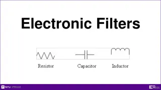
Digital Filters in Signal Processing
Explore the concept of digital filters in signal processing, including realization, MATLAB implementation, transfer function, and pole-zero analysis. Learn how to compute system responses, find transfer functions, and analyze system stability through pole-zero plots.

Download Presentation

Please find below an Image/Link to download the presentation.
The content on the website is provided AS IS for your information and personal use only. It may not be sold, licensed, or shared on other websites without obtaining consent from the author. If you encounter any issues during the download, it is possible that the publisher has removed the file from their server.
You are allowed to download the files provided on this website for personal or commercial use, subject to the condition that they are used lawfully. All files are the property of their respective owners.
The content on the website is provided AS IS for your information and personal use only. It may not be sold, licensed, or shared on other websites without obtaining consent from the author.
E N D
Presentation Transcript
Chapter 6 Digital Filters CEN352, Dr. Nassim Ammour, King Saud University 1
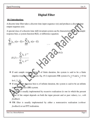
Digital Filtering: Realization Definition: A digital filter is a DSP system, where ? ? ??? y(n) are the DSP system s input and output, respectively. The Digital filter difference equation: Where ?? ??? ?? represent the coefficients of the system. Matlab Implementation: 3-tap (2ndorder) IIR filter CEN352, Dr. Nassim Ammour, King Saud University 2
Example Given the DSP system and the input with initial conditions Compute thesystem response y(n) for 20 samples using MATLAB. Solution: CEN352, Dr. Nassim Ammour, King Saud University 3
Transfer Function If ? ? and ? ? are the input and the output of the Digital filter (DSP) respectively, and ? ? ??? ? ? are their Z-transforms, Differential Equation: Z-Transform Z-Transform: Transfer Function: CEN352, Dr. Nassim Ammour, King Saud University 4
Example: Transfer Function Given a DSP: Find the its transfer function H(z). Z-transform on both sides of the difference equation Z-Transform: factoring Y(z) on the left side and X(z) on the right side Rearrange: Transfer Function: Find the difference equation of the system Given H(z) : Rearrange: Dividing the numerator and denominator by ?2 Differential Equation: Applying the inverse z-transform and using the shift property CEN352, Dr. Nassim Ammour, King Saud University 5
Pole Zero from Transfer Function A digital transfer function can be written in the pole-zero form. The z-plane pole-zero plot is used to investigate characteristics and the stability of the digital system. Relationship of the sampled system in the Laplace domain and its digital system in the z-transform domain mapping: The z-plane is divided into two parts by a unit circle. Each pole is marked on z-plane using the cross symbol x, while each zero is plotted using the small circle symbol o. CEN352, Dr. Nassim Ammour, King Saud University 6
Example: Pole-zero plot Given the digital transfer function: Plot poles and zeros multiplying the numerator and denominator by ?2 ????1 = 0.5 ????1 = 0.6 + ?0.3 ????2 = 0.6 ?0.3 (? ????1) (? ????1)(? ????2) = The system is stable. The zeros do not affect system stability. CEN352, Dr. Nassim Ammour, King Saud University 7
System Stability (Depends on poles location) If the outmost poles of the DSP TF H(z) are inside the unit circle on the z-plane pole-zero plot, then the system is stable. If the outmost poles are first-order poles of the DSP TF H(z) and on the unit circle on the z-plane pole-zero plot, then the system is marginally stable. CEN352, Dr. Nassim Ammour, King Saud University 8
Example: System Stability Sketch the z-plane pole-zero plot and determine the stability for the system: Since the outermost pole is multiple order (2nd order) at z = 1 and is on the unit circle, the system is unstable. CEN352, Dr. Nassim Ammour, King Saud University 9
Digital Filter: Frequency Response From the Laplace transfer function, we can achieve the analog filter frequency response ?(??) by substituting ? = ?? into the transfer function H(s). z = esT s=j = ej T into the Z-transfer function of the system s Similarly, in a DSP system, we substitute transfer function H(z) to acquire the digital frequency response Magnitude frequency response Phase response Putting normalized digital frequency CEN352, Dr. Nassim Ammour, King Saud University 10
Frequency Response Example Given the digital system with a sampling rate of 8,000 Hz, determine the frequency response. Problem Solution z-transform : (on both sides on the difference equation ) Frequency response: transfer function ? = ?? Magnitude frequency response Phase frequency response It is observed that when the frequency increases, the magnitude response decreases. The DSP system acts like a digital low-pass filter, and its phase response is linear. CEN352, Dr. Nassim Ammour, King Saud University 11
Digital Filter: Frequency Response contd. BASIC TYPES OF FILTERING Pass-band Ripple (frequency fluctuation) parameter Stop-band Ripple (frequency fluctuation) parameter High-pass filter (HPF) Stop-band cut-off frequency Pass-band cut-off frequency Low-pass filter (LPF) Matlab: Frequency Response: 12 CEN352, Dr. Nassim Ammour, King Saud University
Digital Filter: Frequency Response contd. BASIC TYPES OF FILTERING Higher stop-band Cut-off frequency Lower stop-band cut-off frequency Lower Pass-band cut-off frequency Higher pass-band Cut-off frequency Band-stop filter (BSF) Band-pass filter (BPF) CEN352, Dr. Nassim Ammour, King Saud University 13


")