Determinants of Total Production in Macroeconomics
An economy's total production of goods and services (GDP) is influenced by the quantity of inputs, known as the Factors of Production, and the ability to transform inputs into output through the production function. The key factors of production are capital and labor, and the production function determines how much output is produced from given amounts of capital and labor. National income is distributed to the factors of production based on factor prices, such as wages for workers and rent for capital owners.

Download Presentation

Please find below an Image/Link to download the presentation.
The content on the website is provided AS IS for your information and personal use only. It may not be sold, licensed, or shared on other websites without obtaining consent from the author.If you encounter any issues during the download, it is possible that the publisher has removed the file from their server.
You are allowed to download the files provided on this website for personal or commercial use, subject to the condition that they are used lawfully. All files are the property of their respective owners.
The content on the website is provided AS IS for your information and personal use only. It may not be sold, licensed, or shared on other websites without obtaining consent from the author.
E N D
Presentation Transcript
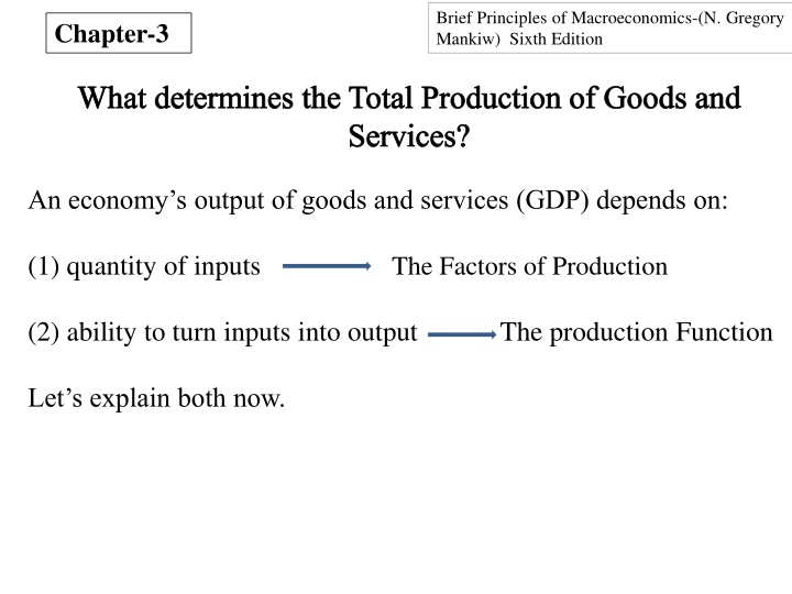
Brief Principles of Macroeconomics-(N. Gregory Mankiw) Sixth Edition Chapter-3 What determines the Total Production of Goods and Services? An economy s output of goods and services (GDP) depends on: (1) quantity of inputs The Factors of Production (2) ability to turn inputs into output The production Function Let s explain both now.
The Factors of Production The factors of production are the inputs used to produce goods and services. The two most important factors of production are capital and labor. In this module, we will take these factors as given (hence the over bar depicting that these values are fixed). K (capital) = K L (labor) = L In this module, we ll also assume that all resources are fully utilized, meaning no resources are wasted.
The Production Function The available production technology determines how much output is produced from given amounts of capital (K) and labor (L). The production function represents the transformation of inputs into outputs. A key assumption is that the production function has constant returns to scale, meaning that if we increase inputs by z, output will also increase by z. We write the production function as: Y = F ( K , L ) given inputs function of Income is To see an example of a production function let s visit Mankiw sBakery
Mankiws Bakery The workers hired to make the bread are its labor. The loaves of bread are its output. The kitchen and its equipment are Mankiw s Bakery capital. Mankiw s Bakery production function shows that the number of loaves produced depends on the amount of the equipment and the number of workers. If the production function has constant returns to scale, then doubling the amount of equipment and the number of workers doubles the amount of bread produced.
The Supply of Goods and Services We can now see that the factors of production and the production functiontogether determine the quantity of goods and services supplied, which in turn equals the economy s output. So, Y = F ( K , L ) = Y In this section, because we assume that capital and labor are fixed, we can also conclude that Y (output) is fixed as well.
How is National Income distributed to the Factors of Production? Recall that the total output of an economy equals total income. Because the factors of production and the production function together determine the total output of goods and services, they also determine national income. Factor Prices The distribution of national income is determined by factor prices. Factor prices are the amounts paid to the factors of production the wages workers earn and the rent the owners of capital collect. Because we have assumed a fixed amount of capital and labor, the factor supply curve is a vertical line. The next slide will illustrate this.
The price paid to any factor of production depends on the supply and demand for that factor s services. Because we have assumed that the supply is fixed, the supply curve is vertical. The demand curve is downward sloping. The intersection of supply and demand determines the equilibrium factor price. FACTOR PRICES Factor price (Wage or rental rate) Factor supply This vertical supply curve is a result of the supply being fixed. Equilibrium factor price Factor demand Quantity of factor
Labor Capital To make a product, the firm needs two factors of production, capital and labor. Let s represent the firm s technology by the usual production function: Y = F (K, L) The firm sells its output at price P, hires workers at a wage W, and rents capital at a rate R.
The goal of the firm is to maximize profit. Profit is revenue minus cost. Revenue equals P Y. Costs include both labor and capital costs. Labor costs equal W L, the wage multiplied by the amount of labor L. Capital costs equal R K, the rental price of capital R times the amount of capital K. Profit = Revenue - Labor Costs - Capital Costs = PY - WL - RK Then, to see how profit depends on the factors of production, we use production function Y = F (K, L) to substitute for Y to obtain: Profit = P F (K, L) - WL - RK This equation shows that profit depends on P, W, R, L, and K. The competitive firm takes the product price and factor prices as given and chooses the amounts of labor and capital that maximize profit.
The Firm's Demand for Factors We know that the firm will hire labor and rent capital in the quantities that maximize profit. But what are those maximizing quantities? To answer this, we must consider the quantity of labor and then the quantity of capital.
The Marginal Product of Labor The marginal product of labor(MPL) is the extra amount of output the firm gets from one extra unit of labor, holding the amount of capital fixed and is expressed using the production function: MPL = F(K, L + 1) - F(K, L). Most production functions have the property of diminishing marginal product: holding the amount of capital fixed, the marginal product of labor decreases as the amount of labor increases. Diminishing Marginal Product of Labor Y The MPL is the change in output when the labor input is increased by 1 unit. As the amount of labor increases, the production function becomes flatter, indicating diminishing marginal product. F (K, L) MPL 1 MPL 1 L
From MPL to Labor Demand When the competitive, profit-maximizing firm is deciding whether to hire an additional unit of labor, it considers how that decision would affect profits. It therefore compares the extra revenue from the increased production that results from the added labor to the extra cost of higher spending on wages. The increase in revenue from an additional unit of labor depends on two variables: the marginal product of labor, and the price of the output. Because an extra unit of labor produces MPL units of output and each unit of output sells for P dollars, the extra revenue is P MPL. The extra cost of hiring one more unit of labor is the wage W. Thus, the change in profit from hiring an additional unit of labor is Profit = Revenue - Cost = (P MPL) - W
Thus, the firms demand for labor is determined by P MPL = W, or another way to express this is MPL = W/P, where W/P is the real wage the payment to labor measured in units of output rather than in dollars. To maximize profit, the firm hires up to the point where the extra revenue equals the real wage. Units of output The MPL depends on the amount of labor. The MPL curve slopes downward because the MPL declines as L increases. This schedule is also the firm s labor demand curve. Real wage Quantity of labor demanded MPL, labor demand Units of labor, L
MPK and Capital Demand The firm decides how much capital to rent in the same way it decides how much labor to hire. The marginal product of capital, or MPK, is the amount of extra output the firm gets from an extra unit of capital, holding the amount of labor constant: MPK = F (K + 1, L) F (K, L). Thus, the MPK is the difference between the amount of output produced with K+1 units of capital and that produced with K units of capital. Like labor, capital is subject to diminishing marginal product. The increase in profit from renting an additional machine is the extra revenue from selling the output of that machine minus the machine s rental price: Profit = Revenue - Cost = (P MPK) R. To maximize profit, the firm continues to rent more capital until the MPK falls to equal the real rental price, MPK = R/P. The real rental price of capital is the rental price measured in units of goods rather than in dollars. The firm demands each factor of production until that factor s marginal product falls to equal its real factor price.
The Division of National Income The income that remains after firms have paid the factors of production is the economic profitof the firms owners. Real economic profit is: Economic Profit = Y - (MPL L) - (MPK K) or to rearrange: Y = (MPL L) - (MPK K) + Economic Profit. Total income is divided among the returns to labor, the returns to capital, and economic profit. How large is economic profit? If the production function has the property of constant returns to scale, then economic profit is zero. This conclusion follows from Euler s theorem, which states that if the production function has constant returns to scale, then F(K,L) = (MPK K) - (MPL L) If each factor of production is paid its marginal product, then the sum of these factor payments equals total output. In other words, constant returns to scale, profit maximization, and competition together imply that economic profit is zero.
Cobb-Douglas Production Function Paul Douglas observed that the division of national income between capital and labor has been roughly constant over time. In other words, the total income of workers and the total income of capital owners grew at almost exactly the same rate. He then wondered what conditions might lead to constant factor shares. Cobb, a mathematician, said that the production function would need to have the property that: Capital Income = MPK K = Labor Income = MPL L = (1- ) Y
Capital Income = MPK K = Y Labor Income = MPL L = (1- ) Y is a constant between zero and one and measures capital and labors share of income. Cobb showed that the function with this property is: F (K, L) = A K L1- A is a parameter greater than zero that measures the productivity of the available technology.
Next, consider the marginal products for the CobbDouglas Production function. The marginal product of labor is: MPL = (1- ) A K L or, MPL = (1- ) Y / L and the marginal product of capital is: MPL = A K -1L1 or, MPK = Y/K Let s now understand the way these equations work.
Properties of Cobb-Douglas Production Function The Cobb Douglas production function has constant returns to scale (remember Mankiw s Bakery). That is, if capital and labor are increased by the same proportion, then output increases by the same proportion as well. Next, consider the marginal products for the Cobb Douglas production function. The MPL : MPL = (1- )Y/L MPK= A/ K The MPL is proportional to output per worker, and the MPK is proportional to output per unit of capital. Y/L is called average labor productivity, and Y/K is called average capital productivity. If the production function is Cobb Douglas, then the marginal productivity of a factor is proportional to its average productivity.
An increase in the amount of capital raises the MPL and reduces the MPK. Similarly, an increase in the parameter MPL = (1- ) A K L or, MPL = (1- ) Y / L and the marginal product of capital is: MPL = A K -1L1 or, MPK = Y/K Let s now understand the way these equations work.
We can now confirm that if the factors (K and L) earn their marginal products, then the parameter indeed tells us how much income goes to labor and capital. The total amount paid to labor is MPL L = (1- ). Therefore (1- ) is labor s share of output Y. Similarly, the total amount paid to capital, MPK K is Y and is capital s share of output. The ratio of labor income to capital income is a constant (1- )/ , just as Douglas observed. The factor shares depend only on the parameter , not on the amounts of capital or labor or on the state of technology as measured by the parameter A. Despite the many changes in the economy of the last 40 years, this ratio has remained about the same (0.7). This division of income is easily explained by a Cobb Douglas production function, in which the parameter is about 0.3.
What Determines the Demand for Goods an Services? Y = C + I + G + NX Total demand for domestic output (GDP) Investment spending by businesses and households Net exports or net foreign demand is composed of Government purchases of goods and services Consumption spending by households We are going to assume our economy is a closed economy, therefore it eliminates the last-term net exports, NX. So, the three components of GDP are Consumption (C), Investment (I) and Government purchases (G). Let s see how GDP is allocated among these three uses.
Consumption (C) Consumption Fuction Yd = Y - T C = C( Yd ) C disposable income consumption spending by households Yd The slope of the consumption function is the MPC.
Marginal Propensity to Consume (MPC) The marginal propensity to consume (MPC) is the amount by which consumption changes when disposable income (Y - T) increases by one dollar. To understand the MPC, consider a shopping scenario. A person who loves to shop probably has a large MPC,let s say ($.99). This means that for every extra dollar he or she earns after tax deductions, he or she spends $.99 of it. The MPC measures the sensitivity of the change in one variable (C) with respect to a change in the other variable (Y - T).
The Investment Function (I) I = I(r) Investment spending depends on real interest rate The quantity of investment depends on the real interest rate, which measures the cost of the funds used to finance investment. When studying the role of interest rates in the economy, economists distinguish between the nominal interest rate and the real interest rate, which is especially relevant when the overall level of prices is changing. The nominal interest rate is the interest rate as usually reported; it is the rate of interest that investors pay to borrow money. The real interest rate is the nominal interest rate corrected for the effects of inflation.
The investment function relates the quantity of investment I to the real interest rate r. Investment depends on the real interest rate because the interest rate is the cost of borrowing. The investment function slopes downward; when the interest rate rises, fewer investment projects are profitable. Real interest rate, r Investment function, I(r) Quantity of investment, I
Government Purchases We take the level of government spending and taxes as given. If government purchases equal taxes minus transfers, then G = T, and the government has a balanced budget. If G > T, then the government is running a budget deficit. If G < T, then the government is running a budget surplus. G = G T = T
What Brings the Supply and Demand for Goods and Services Into Equilibrium? The following equations summarize the discussion of the demand for goods and services: 1) Y = C + I + GDemand for Economy s Output 2) C = C(Y - T) Consumption Function 3) I = I(r) Real Investment Function 4) G = G Government Purchases 5) T = T Taxes The demand for the economy s output comes from consumption, investment, and government purchases. Consumption depends on disposable income; investment depends on the real interest rate; government purchases and taxes are the exogenous variables set by fiscal policy makers.
To this analysis, lets add what weve learned about the supply of goods and services earlier in the module. There we saw that the factors of production and the production function determine the quantity of output supplied to the economy: Y = F (K, L) = Y Now, let s combine these equations describing supply and demand for output Y. Substituting all of our equations into the national income accounts identity, we obtain: Y = C(Y - T) + I(r) + G and then, setting supply equal to demand, we obtain an equilibrium condition: Y = C(Y - T) + I(r) + G This equation states that the supply of output equals its demand, which is the sum of consumption, investment, and government purchases.
Y = C(Y - T) + I(r) + G Notice that the interest rate r is the only variable not already determined in the last equation. This is because the interest rate still has a key role to play: it must adjust to ensure that the demand for goods equals the supply. The greater the interest rate, the lower the level of investment. and thus the lower the demand for goods and services, C + I + G. If the interest rate is too high, investment is too low, and the demand for output falls short of supply. If the interest rate is too low, investment is too high, and the demand exceeds supply. At the equilibrium interest rate, the demand for goods and services equals the supply. Let s now examine how financial markets fit into the story.
The Supply and Demand for Loanable Funds First, rewrite the national income accounts identity as Y - C - G = I. The term Y - C - G is the output that remains after the demands of consumers and the government have been satisfied; it is called national saving or simply, saving (S). In this form, the national income accounts identity shows that saving equals investment. To understand this better, let s split national saving into two parts-- one examining the saving of the private sector and the other representing the saving of the government. (Y - T - C) + (T - G) = I The term (Y - T - C) is disposable income minus consumption, which is private saving. The term (T - G) is government revenue minus government spending, which is public saving. National saving is the sum of private and public saving.
To see how the interest rate brings financial markets into equilibrium, substitute the consumption function and the investment function into the national income accounts identity: Y - C (Y - T) - G = I(r) Next, note that G and T are fixed by policy and Y is fixed by the factors of production and the production function: Y - C (Y - T) - G = I(r) Real interest rate, r S = I(r) The vertical line represents saving-- the supply of loanable funds. The downward-sloping line represents investment--the demand for loanable funds. The intersection determines the equilibrium interest rate. Saving, S Equilibrium interest rate Investment, Saving, I, S S
Changes in Savings: Effects of Fiscal Policy An Increase in Government Purchases: If we increase government purchases by an amount G, the immediate impact is to increase the demand for goods and services by G. But since total output is fixed by the factors of production, the increase in government purchases must be met by a decrease in some other category of demand. Because disposable Y-T is unchanged, consumption is unchanged. The increase in government purchases must be met by an equal decrease in investment. To induce investment to fall, the interest rate must rise. Hence, the rise in government purchases causes the interest rate to increase and investment to decrease. Thus, government purchases are said to crowd out investment. A Decrease in Taxes: The immediate impact of a tax cut is to raise disposable income and thus to raise consumption. Disposable income rises by T, and consumption rises by an amount equal to T times the MPC. The higher the MPC, the greater the impact of the tax cut on consumption. Like an increase in government purchases, tax cuts crowd out investment and raise the interest rate.
Real interest rate, r A reduction in saving, possibly the result of a change in fiscal policy, shifts the saving schedule to the left. The new equilibrium is the point at which the new saving schedule crosses the investment schedule. A reduction in saving lowers the amount of investment and raises the interest rate. Saving, S Desired Investment, I(r) Investment, Saving,I, S S Fiscal policy actions are said to crowd out investment.
Changes in Investment Demand An increase in the demand for investment goods shifts the investment schedule to the right. At any given interest rate, the amount of investment is greater. The equilibrium moves from A to B. Because the amount of saving is fixed, the increase in investment demand raises the interest rate while leaving the equilibrium amount of investment unchanged. Real interest rate, r Saving, S B A I2 I1 Investment, Saving, I, S S Now let s see what happens to the interest rate and saving when saving depends on the interest rate (upward-sloping saving (S) curve).
S(r) Real interest rate, r Upward-sloping savings B I2 A I1 Investment, Saving, I, S When saving is positively related to the interest rate, as shown by the upward-sloping S(r) curve, a rightward shift in the investment schedule I(r), increases the interest rate and the amount of investment. The higher interest rate induces people to increase saving, which in turn allows investment to increase.
Assumptions We have assumed: ignored the role of money, no international trade, the labor force is fully employed, the capital stock, the labor force, and the production technology are fixed ignored the role of short-run sticky prices.


 earn their")

")
")
")


 + I(r) + G")


")