Decision Trees

Decision trees are a popular and successful machine learning technique that iteratively splits a dataset into subsets based on the most informative features. By choosing features constructively, decision trees aim to label each leaf node accurately, making them suitable for both discrete and nominal attributes. This process of constructing smaller and shallower trees helps in generalizing effectively. Various decision tree algorithms, such as ID3, C4.5, and CART, have been developed over the years to enhance their efficiency and handling of real-valued inputs. Understanding the concepts of feature splitting and tree construction is crucial for developing accurate predictive models in decision tree learning.

• Decision Trees
• Machine Learning
• Feature Splitting
• Iterative Approach
• Tree Algorithms

tannehill_k Follow

Uploaded on Feb 22, 2025 | 0 Views

Download Presentation

Please find below an Image/Link to download the presentation.

The content on the website is provided AS IS for your information and personal use only. It may not be sold, licensed, or shared on other websites without obtaining consent from the author.If you encounter any issues during the download, it is possible that the publisher has removed the file from their server.

You are allowed to download the files provided on this website for personal or commercial use, subject to the condition that they are used lawfully. All files are the property of their respective owners.

The content on the website is provided AS IS for your information and personal use only. It may not be sold, licensed, or shared on other websites without obtaining consent from the author.

Presentation Transcript

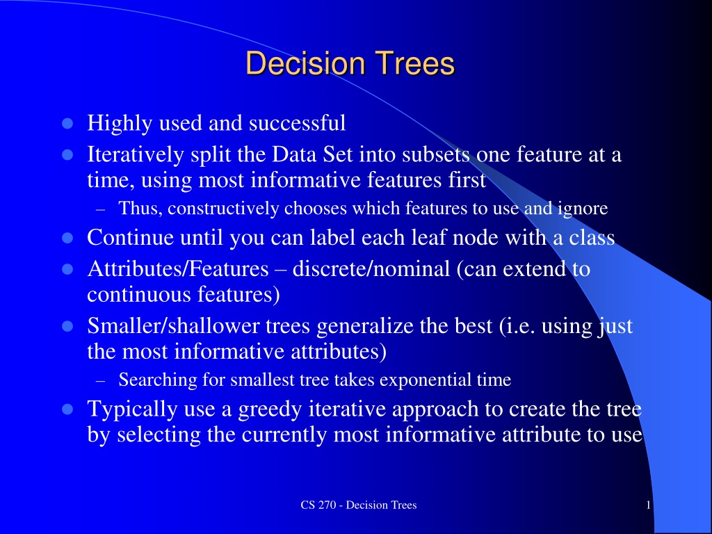
1. Decision Trees Highly used and successful Iteratively split the Data Set into subsets one feature at a time, using most informative features first Thus, constructively chooses which features to use and ignore Continue until you can label each leaf node with a class Attributes/Features discrete/nominal (can extend to continuous features) Smaller/shallower trees generalize the best (i.e. using just the most informative attributes) Searching for smallest tree takes exponential time Typically use a greedy iterative approach to create the tree by selecting the currently most informative attribute to use CS 270 - Decision Trees 1

2. Decision Tree Learning Assume A1 is nominal binary feature (Size: S/L) Assume A2 is nominal 3 value feature (Color: R/G/B) A goal is to get pure leaf nodes. What feature might we split on? R A2 G B A1 S L CS 270 - Decision Trees 2

3. Decision Tree Learning Assume A1 is nominal binary feature (Size: S/L) Assume A2 is nominal 3 value feature (Color: R/G/B) Next step for left and right children? A1 R R G A2 A2 G B B A1 A1 S L S L CS 270 - Decision Trees 3

4. Decision Tree Learning Assume A1 is nominal binary feature (Size: S/L) Assume A2 is nominal 3 value feature (Color: R/G/B) Decision surfaces are axis aligned Hyper-Rectangles A1 A2 R R A2 A2 G G B B A1 A1 S L S L CS 270 - Decision Trees 4

5. Decision Tree Learning Assume A1 is nominal binary feature (Size: S/L) Assume A2 is nominal 3 value feature (Color: R/G/B) Decision surfaces are axis aligned Hyper-Rectangles Label leaf nodes with their majority class A1 A2 R R A2 A2 G G B B A1 A1 S L S L CS 270 - Decision Trees 5

6. Decision Tree Algorithms J Ross Quinlan Australia, ML researcher ID3 (Iterative Dichotimiser 3) 1986 C4.5 Upgrade of ID3, (Version 4.5 written in C) 1993, Handles real valued inputs C5.0 More efficient implementation Leo Breiman - UC Berkeley CART (Classification and Regression Trees) 1984 This is the decision tree approach currently supported in Sklearn Random Forests - 2001 Independently discovered CS 270 - Decision Trees 6

7. ID3/C4.5 Learning Approach S is a set of examples A test on attribute/feature A partitions S into {Si, S2,...,S|A|} where |A| is the number of values A can take on Start with the training set as S and first find a goodA for the root Continue recursively until either all subsets well classified, you run out of attributes, or some stopping criteria is reached CS 270 - Decision Trees 7

8. Which Attribute/Feature to split on Twenty Questions - what are good questions, ones which when asked decrease the information remaining Regularity required What would be good attribute tests for a DT Let s come up with our own approach for scoring the quality of each possible attribute then pick highest CS 270 - Decision Trees 8

9. Which Attribute to split on Twenty Questions - what are good questions, ones which when asked decrease the information remaining Regularity required What would be good attribute tests for a DT Let s come up with our own approach for scoring the quality of each possible attribute then pick highest nmajority ntotal Purity CS 270 - Decision Trees 9

10. Which Attribute to split on Twenty Questions - what are good questions, ones which when asked decrease the information remaining Regularity required What would be good attribute tests for a DT Let s come up with our own approach for scoring the quality of each possible attribute then pick highest nmajority ntotal Want both purity and statistical significance (e.g. SS#) CS 270 - Decision Trees 10

11. Which Attribute to split on Twenty Questions - what are good questions, ones which when asked decrease the information remaining Regularity required What would be good attribute tests for a DT Let s come up with our own approach for scoring the quality of each possible attribute then pick highest nmaj+1 ntotal+|C | nmajority ntotal Want both purity and statistical significance Laplacian, where |C| is the number of output classes CS 270 - Decision Trees 11

12. Which Attribute to split on Twenty Questions - what are good questions, ones which when asked decrease the information remaining Regularity required What would be good attribute tests for a DT Let s come up with our own approach for scoring the quality of each possible attribute then pick highest nmaj+1 ntotal+|C | nmajority ntotal This is just for one node Best attribute will be good across many/most of its partitioned nodes CS 270 - Decision Trees 12

13. Which Attribute to split on Twenty Questions - what are good questions, ones which when asked decrease the information remaining Regularity required What would be good attribute tests for a DT Let s come up with our own approach for scoring the quality of each possible attribute then pick highest nmaj+1 ntotal+|C | nmaj,i+1 ntotal,i+|C | |A| nmajority ntotal ntotal,i ntotal i=1 Now we just try each attribute to see which gives the highest score, and we split on that attribute and repeat at the next level CS 270 - Decision Trees 13

14. Which Attribute to split on Twenty Questions - what are good questions, ones which when asked decrease the information remaining Regularity required What would be good attribute tests for a DT Let s come up with our own approach for scoring the quality of each possible attribute then pick highest nmaj+1 ntotal+|C | nmaj,i+1 ntotal,i+|C | |A| nmajority ntotal ntotal,i ntotal i=1 Sum of Laplacians a reasonable and common approach Another approach (often used by ID3/C4.5): Entropy Just replace Laplacian part with information(node) CS 270 - Decision Trees 14

15. Information Information of a message in bits: I(m) = -log2(pm) If there are 16 equiprobable messages, I for each message is - log2(1/16) = 4 bits If the messages are not equiprobable then could we represent them with less bits? Highest disorder (randomness) requires maximum information If there is a dataset S of c classes, then information for one class is: I(c) = -log2(pc) Total info of the data set is just the sum of the info per class times the proportion of that class |C| Info(S) = Entropy(S) = - log2(pi) pi i=1 CS 270 - Decision Trees 15

16. Information Gain Metric Info(S) is the average amount of information needed to identify the class of an example in set S |C| log2(|C|) - log2(pi) pi Info(S) = Entropy(S) = Info i=1 0 Info(S) log2(|C|), |C| is # of output classes pi is the probability of each output class Expected Information after partitioning using A: |Si| |S |Info(Si) i=1 0 1 prob |A| InfoA(S) = where |A| is # of values for attribute A Mostly pure sets have Info(S) = Entropy(S) 0 Gain(A) = Info(S) - InfoA(S) (i.e. minimize InfoA(S)) Gain/Entropy does not handle the statistical significance issue more on that later CS 270 - Decision Trees 16

17. ID3/C4.5 Learning Algorithm 1. S = Training Set 2. Calculate gain for each remaining attribute: Gain(A) = Info(S) - InfoA(S) 3. Select attribute with highest gain and create a new node for each partition 4. For each new child node if pure (one class), or if no attributes remain, or if stopping criteria met, then label node with majority class and end Stopping criteria include pure enough, too small a number of examples remaining, not enough information gain, max depth reached, etc. else recurse to 2 with remaining attributes and training set |?| ???? ? = ?????2?? ?=1 ? ? |?| ?? ? ?? ? ?????? = ???? ?? = ?????2?? ?=1 ?=1 ?=1 Where S is the remaining training set at the node |A| is the number of attribute values for the feature |C| is the number of output classes for the task 17

18. C4.5 Learning Algorithm 1. S = Training Set 2. Calculate gain for each remaining attribute: Gain(A) = Info(S) - InfoA(S) 3. Select attribute with highest gain and create a new node for each partition 4. For each new child node if pure (one class), or if no attributes remain, or if stopping criteria met (e.g. pure enough, too small a number of examples remaining, not enough information gain, max depth reached), then label node with majority class and end else recurse to 2 with remaining attributes and training set Meat N,Y Crust D,S,T Veg N,Y Quality B,G,Gr |?| ???? ? = ?????2?? Y Thin N Great ?=1 ? N Deep N Bad ? |?| N Stuffed Y Good ?? ? ?? ? ?????? = ???? ?? = ?????2?? Y Stuffed Y Great Y Deep N Good ?=1 ?=1 ?=1 Y Deep Y Great Where S is the remaining training set at the node |A| is the number of attribute values for the feature |C| is the number of output classes for the task N Thin Y Good Y Deep N Good 18 N Thin N Bad

19. Meat N,Y Crust D,S,T Veg N,Y Quality B,G,Gr Example Y Thin N Great |?| N Deep N Bad Where S is the remaining training set at the node |A| is the number of attribute values for the feature |C| is the number of output classes for the task ???? ? = ?????2?? N Stuffed Y Good Y Stuffed Y Great ?=1 Y Deep N Good ? ? |?| Y Deep Y Great ?? ? ?? ? ?????? = ???? ?? = ?????2?? N Thin Y Good Y Deep N Good ?=1 ?=1 ?=1 N Thin N Bad Info(S) = - 2/9 log22/9 - 4/9 log24/9 -3/9 log23/9 = 1.53 Not necessary, but gain can be used as a stopping criteria Starting with all instances, calculate gain for each attribute Let s do Meat: InfoMeat(S) = ? Information Gain is ? CS 270 - Decision Trees 19

20. Meat N,Y Crust D,S,T Veg N,Y Quality B,G,Gr Example Y Thin N Great |?| N Deep N Bad Where S is the remaining training set at the node |A| is the number of attribute values for the feature |C| is the number of output classes for the task ???? ? = ?????2?? N Stuffed Y Good Y Stuffed Y Great ?=1 Y Deep N Good ? ? |?| Y Deep Y Great ?? ? ?? ? ?????? = ???? ?? = ?????2?? N Thin Y Good Y Deep N Good ?=1 ?=1 ?=1 N Thin N Bad Info(S) = - 2/9 log22/9 - 4/9 log24/9 -3/9 log23/9 = 1.53 Not necessary, but gain can be used as a stopping criteria Starting with all instances, calculate gain for each attribute Let s do Meat: InfoMeat(S) = 4/9 (-2/4log22/4 - 2/4 log22/4 - 0 log20/4) + 5/9 (-0/5 log20/5 - 2/5 log22/5 - 3/5 log23/5) = .98 Information Gain is 1.53 - .98 = .55 CS 270 - Decision Trees 20

21. Meat N,Y Crust D,S,T Veg N,Y Quality B,G,Gr *Challenge Question* Y Thin N Great |?| N Deep N Bad Where S is the remaining training set at the node |A| is the number of attribute values for the feature |C| is the number of output classes for the task ???? ? = ?????2?? N Stuffed Y Good Y Stuffed Y Great ?=1 Y Deep N Good ? ? |?| ?? ? ?? ? Y Deep Y Great ?????? = ???? ?? = ?????2?? N Thin Y Good ?=1 ?=1 ?=1 Y Deep N Good N Thin N Bad What is the information for crust InfoCrust(S) : A. .98 B. 1.35 C. .12 D. 1.41 E. None of the Above Is it a better attribute to split on than Meat? CS 270 - Decision Trees 21

22. Meat N,Y Crust D,S,T Veg N,Y Quality B,G,Gr Decision Tree Example Y Thin N Great N Deep N Bad |?| N Stuffed Y Good ???? ? = ?????2?? Y Stuffed Y Great ?=1 Y Deep N Good Y Deep Y Great ? ? |?| ?? ? ?? ? N Thin Y Good ?????? = ???? ?? = ?????2?? Y Deep N Good ?=1 ?=1 ?=1 N Thin N Bad InfoMeat(S) = 4/9 (-2/4log22/4 - 2/4 log22/4 - 0 log20/4) + 5/9 (-0/5 log20/5 - 2/5 log22/5 - 3/5 log23/5) = .98 InfoCrust(S) = 4/9 (-1/4log21/4 - 2/4 log22/4 - 1/4 log21/4) + 2/9 (-0/2 log20/2 - 1/2 log21/2 - 1/2 log21/2) + 3/9 (-1/3 log21/3 - 1/3 log21/3 - 1/3 log21/3) = 1.41 Meat leaves less info (higher gain) and thus is the better of these two CS 270 - Decision Trees 22

23. Meat N,Y Crust D,S,T Veg N,Y Quality B,G,Gr Decision Tree Homework Y Thin N Great N Deep N Bad |?| N Stuffed Y Good ???? ? = ?????2?? Y Stuffed Y Great ?=1 Y Deep N Good Y Deep Y Great ? ? |?| ?? ? ?? ? N Thin Y Good ?????? = ???? ?? = ?????2?? Y Deep N Good ?=1 ?=1 ?=1 N Thin N Bad Finish the first level, find the best attribute and split Then find the best attribute for the left most node at the second level and split the node accordingly Assume sub-nodes are sorted alphabetically left to right by attribute Label any leaf nodes with their majority class You could continue with the other nodes to get more practice CS 270 - Decision Trees 23

24. C4.5 Notes Attributes which best discriminate between classes are chosen If the same ratios are found in a partitioned set, then gain is 0 Complexity: At each tree node with a set of instances the work is O(|Instances| * |remaining attributes|), which is Polynomial Total complexity is empirically polynomial O(|TrainingSet| * |attributes| * |nodes in the tree|) where the number of nodes is bound by the number of attributes and can be kept smaller through stopping criteria, etc. CS 270 - Decision Trees 24

25. Decision Tree Overfit Avoidance Noise can cause inability to converge 100% or can lead to overly complex decision trees (overfitting). Thus, we usually allow leafs with multiple classes. Can select the majority class as the output, or output a confidence vector Also, may not have sufficient attributes to perfectly divide data Even if no noise, statistical chance can lead to overfit, especially when the training set is not large. (e.g. some irrelevant attribute may happen to cause a perfect split in terms of info gain on the training set, but will generalize poorly) Common approach is to not split when the number of examples at the node are less than a threshold and just label this leaf node with its majority class early stopping Could use a validation set and only add a new node if improvement (or no decrease) in accuracy on the validation set checked independently at each branch of the tree using data set from parent But shrinking data problem with decision trees CS 270 - Decision Trees 25

26. C4.5 Overfit Avoidance Use Chi-square test to decide confidence in whether attribute is irrelevant. Approach used in original ID3. (Takes amount of data into account) C4.5 allows tree to be changed into a rule set. Rules can then be pruned in other ways. If testing a truly irrelevant attribute, then the class proportion in the partitioned sets should be similar to the initial set, with a small info gain. Could only split if information gain exceeds some threshold. However, in DTs, this type of early stopping can miss later higher order combinations that would have helped. C4.5 handles overfit by first filling out complete tree and then pruning any nodes which don t help validation set accuracy CS 270 - Decision Trees 26

27. Reduced Error Pruning Pruning a full tree (one where all possible nodes have been added) Prune any nodes which would not hurt accuracy Could allow some higher order combinations that would have been missed with early stopping Can simultaneously consider all nodes for pruning rather than just the current frontier 1. Train tree out fully (empty or consistent partitions or no more attributes) 2. For EACH non-leaf node, test accuracy on a validation set for a modified tree where the sub-trees of the node are removed and the node is assigned the majority class based on the instances it represents from the training set 3. Keep pruned tree which does best on the validation set and does at least as well as the current tree on the validation set 4. Repeat until no pruned tree does as well as the current tree CS 270 - Decision Trees 27

28. Reduced Error Pruning Example CS 270 - Decision Trees 28

29. Missing Values: C4.5 Approach Can use any of the methods we discussed previously new attribute value very natural and effective with typical nominal data Another approach, particular to decision trees: When arriving at an attribute test for which the attribute is missing do the following: Each branch has a probability of being taken based on what percentage of examples at that parent node have the branch's value for the missing attribute Take all branches, but carry a weight representing that probability. These weights could be further modified (multiplied) by other missing attributes in the current example as they continue down the tree. Thus, a single instance gets broken up and appropriately distributed down the tree but its total weight throughout the tree will always sum to 1 Results in multiple active leaf nodes. For execution, set output as leaf with highest weight, or sum weights for each output class, and output the class with the largest sum, (or output the class confidence). During learning, scale instance contribution by instance weights. This approach could also be used for labeled probabilistic inputs with subsequent probabilities tied to outputs CS 270 - Decision Trees 29

30. Real Valued Features C4.5: Continuous data is handled by testing all n-1 possible binary thresholds for each continuous feature to see which gives best information gain. The split point with highest gain gives the score for that feature which then competes with all other features. More efficient to just test thresholds where there is a change of classification. Is binary split sufficient? Attribute may need to be split again lower in the tree, no longer have a strict depth bound CS 270 - Decision Trees 30

31. DT Interpretability Intelligibility of DT When trees get large, intelligibility drops off C4.5 rules - transforms tree into prioritized rule list with default (most common output for examples not covered by rules). It does simplification of superfluous attributes by greedy elimination strategy (based on statistical error confidence as in error pruning). Prunes less productive rules within rule classes How critical is intelligibility in general? Will truly hard problems have a simple explanation? CS 270 - Decision Trees 31

32. Information gain favors attributes with many attribute values If A has random values (SS#), but ends up with only 1 example in each partition, it would have maximum information gain, though a terrible choice. Occam s razor would suggest seeking trees with less overall nodes. Thus, attributes with less possible values might be given some kind of preference. Binary attributes (CART) are one solution, but lead to deeper trees, and somewhat higher complexity in possible ways of splitting attributes Can use a penalty for attributes with many values such as Laplacian: (nc+1)/(n+|C|)), though real issue is splits with little data Gain Ratio is the approach used in original ID3/C4.5 CS 270 - Decision Trees 32

33. C4.5 - Gain Ratio Criteria The main problem is splits with little data What might we do? Laplacian or variations common: (nc+1)/(n+|C|) where nc is the majority class and |C| is the number of output classes |A| Si |S |log 2Si - Gain Ratio: Split information of an attribute SI(A) = |S | i=1 What is the information content of splitting on attribute A - does not ask about output class SI(A) or Split information is larger for a) many valued attributes and b) when A evenly partitions data across values. SI(A) is log2(|A|) when partitions are all of equal size. Want to minimize "waste" of this information. When SI(A) is high then Gain(A) should be high to take advantage. Maximize Gain Ratio: Gain(A)/SI(A) However, somewhat unintuitive since it also maximizes ratio for trivial partitions (e.g. |S| |Si| for one of the partitions), so.... Gain must be at least average of different A before considering gain ratio, so that very small SI(A) does not inappropriately skew Gain ratio. CS 270 - Decision Trees 33

34. CART Classification and Regression Trees Binary Tree Considers all possible splits, also with nominals Color = blue (vs not blue), Height >= 60 inches Recursive binary splitting Same feature could be split multiple times No preset limit on depth like with C4.5 with nominal features Does avoid bushy split problem of C4.5 (SS#) CS 270 - Decision Trees 34

35. Titanic Survival Dataset CS 270 - Decision Trees 35

36. Gini Impurity For classification CART uses Gini impurity for node score |?|?? 2 Gini score for a node is: ? = 1 ?=1 pi is percentage of leaf's instances with output class i Best case is 0 (all one class), worse is 1-1/|C| (equal percentage of each) Total score for a given split is the weighted sum of the two sub-node G s CS 270 - Decision Trees 36

37. Purity vs Gini Purity vs Entropy Purity vs Gini examples Just consider Gini purity part |?| nmajority ntotal 2 ? = 1 ?? ?=1 If all of one class they are the same, (10, 0, 0) both give 1 If (5, 5) both give .5 Which split would we prefer between (6, 4, 0) and (6, 2, 2)? Purity and Gini scores? Big win for later in the decision tree. Entropy has the same advantages as Gini Gini Impurity vs Entropy They are similar in terms of the values they return and often lead to the same overall results, though they differ in some situations Gini avoids the log computation which some like CS 270 - Decision Trees 37

38. CART Overfit Avoidance Most common approach is to stop when there are only a small number of examples at a node which is a type of early stopping Hyperparameter - don t split further when less than (e.g. 5, 10) Can also constrain the tree to be smaller (max nodes, max depth, etc.) but could cause underfit! (like using less hidden nodes in a MLP Can use pruning after full learning for regularization Sklearn has a different pruning algorithm for CART than Reduced Error Pruning CS 270 - Decision Trees 38

39. CART Regression Regression Tree The output value for a leaf is just the average of the outputs of the instances represented by that leaf Could adjust for outliers, etc. Could do the same with C4.5 For regression the score for a node is not GINI impurity, but is the SSE of instances represented by the node The feature score for a potential split is the weighted sum of the two child nodes scores (SSE) Then, just like with classification, we choose the lowest score amongst all possible feature splits As long as there is significant variance in node examples, splitting will continue CS 270 - Decision Trees 39

40. Decision Trees - Conclusion Good Empirical Results Comparable application robustness and accuracy with MLPs Fast learning since no iterations MLPs can be more natural with continuous inputs, while DT natural with nominal inputs One of the most used and well known of current symbolic systems Can be used as a feature filter for other algorithms Attributes higher in the tree are best, those rarely used can be dropped Higher order attribute tests - C4.5 can do greedy merging into value sets, based on whether that improves gain ratio. Executes the tests at each node expansion allowing different value sets at different parts of the tree. Exponential time based on order. CS 270 - Decision Trees 40

41. Decision Tree Lab Nominals SK CART only accepts numeric features - Fits CART fine since that is how CART thinks of nominal features anyways, breaking them into separate one-hot features for each possible feature value So a nominal attribute Color with 3 attribute values (Red, Green, Blue), would be represented as 3 one-hot features Is-Red, Is-Green, Is-Blue Binary features can just be represented as 0/1 Note that Color could appear multiple times in a branch unlike in C4/5. A not Is-Read branch could later consider Is-Blue or Is-Green. CS 270 - Decision Trees 41

42. Midterm and Class Business Double check that all is correct with groups and e-mail me if not E-mail me for group member contact info if needed Working on DT lab early is great exam prep Midterm Exam overview See Study Guide CS 270 - Decision Trees 42