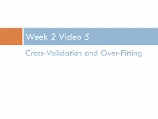
Cross-Validation in Machine Learning

Intro to machine learning:
Cross Validation
Basics of Statistics
Mean Squared Error and Root Mean Squared Error
Mean Squared Error (MSE)
•
Quantify the extent to which the predicted response value for a
given observation is close to the true response value for that
observation.
•
MSE will be small if the
predicted responses are very close to the
true responses
•
RMSE: Root Mean Square Error is the square root of MSE. This
value represents the average distance of a data point from the
fitted model.
Why we use the Validation Set Approach
•
It is one of the techniques used to test the effectiveness of a
machine learning models, it is also a resampling procedure used
to evaluate a model if we have limited data.
•
Minimize the influence of overfitting
•
A model would overfit when being trained on the training set
•
Check for the accuracy on future predictions
•
Since the data are separated into training set and validation set
Example of Overfitting
If we want the f value at x=-5,
the prediction would be around
12, while the actual output
should be around negative 12.
A good statistical model should
not only be accurate for present
data, but also should be
accurate for the future
prediction.
The Validation Set Approach
•
Randomly divides the available set of observations into two parts:
(a)
A training set: the set that the model is fitted on
(b)
A validation set: the set that evaluates the performance of the model
•
Large variability: Repeat the process of the process
a different estimate for the
test MSE will be obtained
•
MSE is used as a measure of validation set error
•
The validation set error rates that result from fitting various regression models on the
training sample and evaluating their performance on the validation sample.
•
Drawbacks:
(a)
Validation estimate of the test error rate highly variable
•
This approach depends highly on how observations are included in the training set and the
validation set.
(b)
Overestimation of the test error rate
•
By nature of this approach, some observations will not be included in the training set. Since
statistical models perform worse when trained on fewer observation, this will lead to an
overestimation.
•
By reducing the training data, we risk losing important patterns/ trends in data set, which in
turn increases error induced by bias.
K-fold Cross Validation
•
Randomly dividing the set of the observations into k groups of
approximately equal size
•
Validation set: the first fold
•
Training set: the remaining (k – 1) folds
•
Procedure repeated k times; each time a different group of
observations is treated as a validationset
•
In practice, k = 5 or k = 10 is typically used
•
Advantage: computation-friendly
•
Disadvantage: variability
Graph Illustration of 5-fold CV
This is an example of a 5-fold
cross validation.
The training set is shown in blue,
while the validation set is shown
in beige.
A set of n observations is
randomly split into five non-
overlapping groups. Each of
these fifths acts as a validation
set, and the remainder as a
training set. The test error is
estimated by averaging the five
resulting MSE estimates.
Comparison between
Leave-One-Out Cross Validation
and K-fold CV
•
Leave-One-Out Cross Validation: the extreme case of k-fold CV where k = n.
•
Recall: K-fold CV with k<n has a computational advantage to LOOCV; K-fold
CV often gives more accurate estimates of the test error rate than LOOCV
(bias-variance tradeoff).
•
Note that we are averaging the outputs of k fitted models that are somewhat less
correlated with each other, since the overlap between the training sets in each model is
smaller.
•
The mean of many highly correlated quantities has higher variance than does the mean
of many quantities that are not highly correlated---the test error estimate resulting
from LOOCV tends to have higher variance than does the test error estimate resulting
from k-fold CV.
•
LOOCV has low bias and high variance
•
Low bias: it
will give approximately unbiased estimates of the test error, since each
training set contains n − 1 observations, which is almost as many as the number of
observations in the full data set.
•
High variance:
Averaging the outputs of n fitted models, each of which is trained on an
almost identical set of observations—outputs highly positively correlated with each
other.
R Explanation of Cross Validation
R Explanation of Cross Validation
This is an application of a 10-fold cross validation and a 5-fold
cross validation. (for comparison)
In this application, we consider an example with wine and its
properties, for instance pH, density and amount of alcohol
contained.
We want our model to predict quality given other 11 properties.
Input data and general view
•
We first have a general view of
all the data we have:
str(wine)
summary(wine)
As we can see, we have 4898
observations and 12 variables.
Each variable is a property of the
wine. (including the quality)
Fit a large model
initial.large.model = lm(quality ~ . , data = wine)
Now we have a linear model with 11 variables, and 12 coefficients
are shown in the graph.
RMSE = 0.7504359
Comparison of observed value and predicted value
•
Let us look at a few lines of observed vs.
predicted values.
head(cbind(observed.value,
predicted.values))
tail(cbind(observed.value,
predicted.values))
•
We can see from the output that
though the predicted values are
generally close to observed values, the
difference is not very small.
10-fold Cross Validation
•
First, we need to pick each row randomly in one of the ten folds.
•
Note that the fold may not contain equal number of rows.
•
This is okay as long as we have a decent amount of data.
no.of.folds = 10
•
Here we set the number of folds to 10.
set.seed(778899)
•
This function sets the random number generator to a starting value. Thus,
each time we run this program we will get the same data.
index.values = sample(1:no.of.folds, size = dim(wine)[1], replace = TRUE)
head(index.values)
table(index.values)/dim(wine)[1]
10-fold Cross Validation
test.mse = rep(0, no.of.folds)
test.mse
for (i in 1:no.of.folds)
{index.out = which(index.values == i)### These are the indices of the rows that will be left out.
left.out.data = wine[ index.out, ]
### This subset of the data is left out. (about 1/10)
left.in.data = wine[ -index.out, ]
### This subset of the data is used to get our regression model. (about 9/10)
tmp.lm = lm(quality ~ ., data = left.in.data)
### Perform regression using the data that is left in.
tmp.predicted.values = predict(tmp.lm, newdata = left.out.data)
### Predict the y values for the data that was left out
test.mse[i] = mean((left.out.data[,12] - tmp.predicted.values)^2)
### Get one of the test.mse's
}
10-fold Cross Validation
•
Now we would like to know how this cross validation works in
terms of MSE:
•
We can see that this RMSE is slightly higher than the one
calculated with the large model (0.7504359).
•
The actual error is close to 0.7544408, which means if new data is
given the error will be 0.7544408, rather than 0.7504359.
5-fold Cross Validation
•
Similar procedure is done for a 5-fold cross validation:
Simply change
no.of.folds = 5
And we have:
Note that the RMSE of 5-fold CV is larger than 10-fold CV and the
large model.
The higher value of K leads to less biased and larger variance
model, which might lead to overfit.
Thank you for reading!
Cross-validation is a crucial technique in machine learning used to evaluate model performance. It involves dividing data into training and validation sets to prevent overfitting and assess predictive accuracy. Mean Squared Error (MSE) and Root Mean Squared Error (RMSE) quantify prediction accuracy, while the Validation Set Approach minimizes overfitting and assesses future predictions. However, there are drawbacks like variability and potential overestimation of error rate. K-fold Cross Validation is another method commonly used in model evaluation.

Download Presentation

Please find below an Image/Link to download the presentation.
The content on the website is provided AS IS for your information and personal use only. It may not be sold, licensed, or shared on other websites without obtaining consent from the author.If you encounter any issues during the download, it is possible that the publisher has removed the file from their server.
You are allowed to download the files provided on this website for personal or commercial use, subject to the condition that they are used lawfully. All files are the property of their respective owners.
The content on the website is provided AS IS for your information and personal use only. It may not be sold, licensed, or shared on other websites without obtaining consent from the author.
E N D
Presentation Transcript
Intro to machine learning: Cross Validation
Basics of Statistics Mean Squared Error and Root Mean Squared Error
Mean Squared Error (MSE) Quantify the extent to which the predicted response value for a given observation is close to the true response value for that observation. MSE will be small if the predicted responses are very close to the true responses RMSE: Root Mean Square Error is the square root of MSE. This value represents the average distance of a data point from the fitted model.
Why we use the Validation Set Approach It is one of the techniques used to test the effectiveness of a machine learning models, it is also a resampling procedure used to evaluate a model if we have limited data. Minimize the influence of overfitting A model would overfit when being trained on the training set Check for the accuracy on future predictions Since the data are separated into training set and validation set
Example of Overfitting If we want the f value at x=-5, the prediction would be around 12, while the actual output should be around negative 12. A good statistical model should not only be accurate for present data, but also should be accurate for the future prediction.
The Validation Set Approach Randomly divides the available set of observations into two parts: (a) A training set: the set that the model is fitted on (b) A validation set: the set that evaluates the performance of the model Large variability: Repeat the process of the process a different estimate for the test MSE will be obtained MSE is used as a measure of validation set error The validation set error rates that result from fitting various regression models on the training sample and evaluating their performance on the validation sample. Drawbacks: (a) Validation estimate of the test error rate highly variable This approach depends highly on how observations are included in the training set and the validation set. (b) Overestimation of the test error rate By nature of this approach, some observations will not be included in the training set. Since statistical models perform worse when trained on fewer observation, this will lead to an overestimation. By reducing the training data, we risk losing important patterns/ trends in data set, which in turn increases error induced by bias.
K-fold Cross Validation Randomly dividing the set of the observations into k groups of approximately equal size Validation set: the first fold Training set: the remaining (k 1) folds Procedure repeated k times; each time a different group of observations is treated as a validationset In practice, k = 5 or k = 10 is typically used Advantage: computation-friendly Disadvantage: variability
Graph Illustration of 5-fold CV This is an example of a 5-fold cross validation. The training set is shown in blue, while the validation set is shown in beige. A set of n observations is randomly split into five non- overlapping groups. Each of these fifths acts as a validation set, and the remainder as a training set. The test error is estimated by averaging the five resulting MSE estimates.
Comparison between Leave-One-Out Cross Validation and K-fold CV Leave-One-Out Cross Validation: the extreme case of k-fold CV where k = n. Recall: K-fold CV with k<n has a computational advantage to LOOCV; K-fold CV often gives more accurate estimates of the test error rate than LOOCV (bias-variance tradeoff). Note that we are averaging the outputs of k fitted models that are somewhat less correlated with each other, since the overlap between the training sets in each model is smaller. The mean of many highly correlated quantities has higher variance than does the mean of many quantities that are not highly correlated---the test error estimate resulting from LOOCV tends to have higher variance than does the test error estimate resulting from k-fold CV. LOOCV has low bias and high variance Low bias: it will give approximately unbiased estimates of the test error, since each training set contains n 1 observations, which is almost as many as the number of observations in the full data set. High variance: Averaging the outputs of n fitted models, each of which is trained on an almost identical set of observations outputs highly positively correlated with each other.
R Explanation of Cross Validation This is an application of a 10-fold cross validation and a 5-fold cross validation. (for comparison) In this application, we consider an example with wine and its properties, for instance pH, density and amount of alcohol contained. We want our model to predict quality given other 11 properties.
Input data and general view We first have a general view of all the data we have: str(wine) summary(wine) As we can see, we have 4898 observations and 12 variables. Each variable is a property of the wine. (including the quality)
Fit a large model initial.large.model = lm(quality ~ . , data = wine) Now we have a linear model with 11 variables, and 12 coefficients are shown in the graph. RMSE = 0.7504359
Comparison of observed value and predicted value Let us look at a few lines of observed vs. predicted values. head(cbind(observed.value, predicted.values)) tail(cbind(observed.value, predicted.values)) We can see from the output that though the predicted values are generally close to observed values, the difference is not very small.
10-fold Cross Validation First, we need to pick each row randomly in one of the ten folds. Note that the fold may not contain equal number of rows. This is okay as long as we have a decent amount of data. no.of.folds = 10 Here we set the number of folds to 10. set.seed(778899) This function sets the random number generator to a starting value. Thus, each time we run this program we will get the same data. index.values = sample(1:no.of.folds, size = dim(wine)[1], replace = TRUE) head(index.values) table(index.values)/dim(wine)[1]
10-fold Cross Validation test.mse = rep(0, no.of.folds) test.mse for (i in 1:no.of.folds) {index.out ### These are the indices of the rows that will be left out. left.out.data = wine[ index.out, ] ### This subset of the data is left out. (about 1/10) left.in.data = wine[ -index.out, ] ### This subset of the data is used to get our regression model. (about 9/10) tmp.lm = lm(quality ~ ., data = left.in.data) ### Perform regression using the data that is left in. tmp.predicted.values = predict(tmp.lm, newdata = left.out.data) ### Predict the y values for the data that was left out test.mse[i] = mean((left.out.data[,12] - tmp.predicted.values)^2) ### Get one of the test.mse's } = which(index.values == i)
10-fold Cross Validation Now we would like to know how this cross validation works in terms of MSE: We can see that this RMSE is slightly higher than the one calculated with the large model (0.7504359). The actual error is close to 0.7544408, which means if new data is given the error will be 0.7544408, rather than 0.7504359.
5-fold Cross Validation Similar procedure is done for a 5-fold cross validation: Simply change no.of.folds = 5 And we have: Note that the RMSE of 5-fold CV is larger than 10-fold CV and the large model. The higher value of K leads to less biased and larger variance model, which might lead to overfit.


")