Confidence Intervals in Statistical Inference
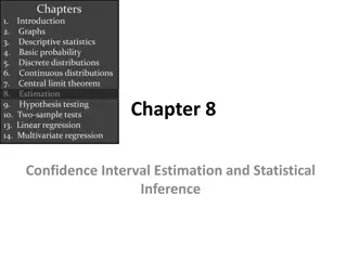
Chapter 8: Confidence Intervals based
on a Single Sample
http://pballew.blogspot.com/2011/03/100-confidence-interval.html
Statistical Inference
2
Sampling
Sampling Variability
What would happen if we took many samples?
3
8.1: Point Estimation - Goals
•
Be able to differentiate between an estimator and an
estimate.
•
Be able to define what is meant by a unbiased or
biased estimator and state which is better in general.
•
Be able to determine from the pdf of a distribution,
which estimator is better.
•
Be able to define MVUE (minimum-variance unbiased
estimator).
•
Be able to state what estimator we will be using for the
rest of the book and why we are using the estimator.
4
Definition: Point Estimate
A
point estimate
of a population parameter,
θ
, is
a single number computed from a sample,
which serves as a best guess for the
parameter.
Definition: Estimator and Estimate
1.
An
estimator
is a statistic of interest, and is
therefore a random variable. An estimator
has a distribution, a mean, a variance, and a
standard deviation.
2.
An
estimate
is a specific value of an
estimator.
What Statistic to Use?
7
Fig. 8.1
Biased/Unbiased Estimator
8
Unbiased Estimators
http://www.weibull.com/DOEWeb/unbiased_and_biased_estimators.htm
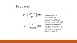
Estimators with Minimum Variance
Minimum Variance Unbiased Estimator
Estimators with Minimum Variance
8.2: A confidence interval (CI) for a
population mean when
is known- Goals
•
State the assumptions that are necessary for a
confidence interval to be valid.
•
Be able to construct a confidence level C CI for
for a
sample size of n with known
σ
(critical value).
•
Explain how the width changes with confidence level,
sample size and sample average.
•
Determine the sample size required to obtain a
specified width and confidence level C.
•
Be able to construct a confidence level C confidence
bound
for
for a sample size of n with known
σ
(critical
value).
•
Determine when it is proper to use the CI.
13
Assumptions for Inference
1.
We have an SRS from the population of
interest.
2.
The variable we measure has a Normal
distribution (or approximately normal
distribution) with mean
and standard
deviation
σ
.
3.
We don’t know
a.
but we do know
σ
(Section 8.2)
b.
We do not know
σ
(Section 8.3)
14
σ
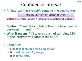
Definition of CI
•
A
confidence interval
(CI) for a population
parameter is an interval of values constructed
so that, with a specified degree of confidence,
the value of the population parameter lies in
this interval.
•
The
confidence coefficient
, C,
is the
probability the CI encloses the population
parameter in repeated samplings.
•
The
confidence level
is the confidence
coefficient expressed as a percentage.
15
z
α
/2
z
α
/2
is a value on the measurement axis in a
standard normal distribution such that
P
(
Z
≥
z
α
/2
) =
α
/2
.
P
(
Z
-
z
α
/2
) =
α
/2
P
(
Z
z
α
/2
) = 1-
α
/2
16
Confidence Interval: Definition
17
Example: Confidence Interval 1
Suppose we obtain a SRS of 100 plots of corn
which have a mean yield (in bushels) of
x̅ = 123.8 and a standard deviation of
σ
= 12.3.
What are the plausible values for the
(population) mean yield of this variety of corn
with a 95% confidence level?
18
Confidence Interval: Definition
19
Confidence Interval
20
Confidence Interval
21
Interpretation of CI
•
The population parameter,
µ
,
is fixed.
•
The confidence interval varies from sample to
sample.
•
It is correct to say “We are 95% confident that
the interval captures the true mean
µ
.”
•
It is incorrect to say “We are 95% confident
µ
lies in the interval.”
22
Interpretation of CI
•
The confidence coefficient, a probability, is a
long-run limiting relative frequency.
•
In repeated samples, the proportion of
confidence intervals that capture the true
value of
µ
approaches the confidence
coefficient.
23
Interpretation
of CI
24
x
CI conclusion
We are
95
% (
C
%) confident that the population
(true) mean of
[…]
falls in the interval
(a,b)
[or is
between
a and b
].
We are
95
% confident that the population (true)
mean
yield of this type of corn
falls in the
interval
(121.4, 126.2)
[or is between
121.4
and
126.2 bushels
].
25
Table III (end of table)
26
Confidence Interval: Definition
27
Table III (end of table)
28
Example: Confidence Interval 2
An experimenter is measuring the lifetime of a
battery. The distribution of the lifetimes is
positively skewed similar to an exponential
distribution. A sample of size 196 produces
x̅ = 2.268. The population standard deviation
is known to be 1.935 for this population.
a) Find and interpret the 95% Confidence
Interval.
b) Find and interpret the 90% Confidence
Interval.
c) Find and interpret the 99% Confidence
Interval.
29
Example: Confidence Interval 2 (cont)
We are 95% confident that the population mean
lifetime of this battery falls in the interval
(1.997, 2.539).
We are 90% confident that the population mean
lifetime of this battery falls in the interval
(2.041, 2.495).
We are 99% confident that the population mean
lifetime of this battery falls in the interval
(1.912, 2.624).
30
How Confidence Intervals Behave
31
Example: Confidence Level & Precision
The following are two CI’s having a confidence
level of 90% and the other has a level of 95%
level: (-0.30, 6.30) and (-0.82,6.82).
Which one has a confidence level of 95%?
32
Impact of Sample Size
33
Example: Confidence Interval 2 (cont.)
An experimenter is measuring the lifetime of a
battery. The distribution of the lifetimes is positively
skewed similar to an exponential distribution. A
sample of size 196 produces x̅ = 2.268 and s = 1.935.
a) Find the Confidence Interval for a 95% confidence
level.
b) Find the Confidence Interval for the 90%
confidence level.
c) Find the Confidence Interval for the 99% confidence
level.
d) What sample size would be necessary to obtain a
margin of error of 0.2 at a 99% confidence level?
34
Practical Procedure
1.
Plan your experiment to obtain the lowest
possible.
2.
Determine the confidence level that you
want.
3.
Determine the largest possible width that is
acceptable.
4.
Calculate what n is required.
5.
Perform the experiment.
35
Confidence Bound
36
Example: Confidence Bound
The following is summary data on shear strength
(kip) for a sample of 3/8-in. anchor bolts: n =
78, x̅ = 4.25,
= 1.30.
Calculate a lower confidence bound using a
confidence level of 90% for the true average
shear strength.
We are 90% confident that the true average
shear strength is greater than ….
37
Summary CI
38
Cautions
1.
The data must be an SRS from the
population.
2.
Be careful about outliers.
3.
You need to know the sample size.
4.
You are assuming that you know
σ
.
5.
The margin of error covers only random
sampling errors!
39
Conceptual Question
One month the actual unemployment rate in the
US was 8.7%. If during that month you took an
SRS of 250 people and constructed a 95% CI to
estimate the unemployment rate, which of
the following would be true:
1) The center of the interval would be 0.087
2) A 95% confidence interval estimate contains
0.087.
3) If you took 100 SRS of 250 people each, 95%
of the intervals would contain 0.087.
40
8.3: Inference for the Mean of a Population
- Goals
•
Be able to construct a level C confidence interval
(without knowing
) and interpret the results.
•
Be able to determine when the t procedure is valid.
41
Assumptions for Inference
1.
We have an SRS from the population of
interest.
2.
The variable we measure has a Normal
distribution (or approximately normal
distribution) with mean
and standard
deviation
σ
.
3.
We don’t know
a.
but we do know
σ
(Section 8.2)
b.
We do not know
σ
(Section 8.3)
42
σ
Shape of t-distribution
http://upload.wikimedia.org/wikipedia/commons/thumb/4/41/Student_t_pdf.svg/1000
px-Student_t_pdf.svg.png
43
t Critical Values
t
,
is a critical value for a t distribution with
degrees of freedom
P(T ≥ t
,
) =
44
t-Table
(Table V)
45
Table III vs. Table V
46
Example: t critical values
What is the t critical value for the following:
a)
Central area = 0.95, df = 10
b)
Central area = 0.95, df = 60
c)
Central area = 0.95, df = 100
d)
Central area = 0.95, z curve
e)
Upper area = 0.99, df = 10
f)
Lower area = 0.99, df = 10
47
Summary CI – t distribution
48
Example: t-distribution
We were curious about what the average time
(hours per month) that students spent watching
videos on cell phones month U.S. College
students. We took an SRS of size 41 and
determined a sample mean of 7.16 and a
sample standard deviation of 3.56.
a) Determine the 95% CI.
b) What sample size is required to obtain a half
width of 0.9 hours/month at a 95%
confidence level?
49
Robustness of the t-procedure
•
A statistical value or procedure is
robust
if the
calculations required are insensitive to
violations of the condition.
•
The t-procedure is robust against normality.
–
n < 15 : population distribution should be
close to normal.
–
15 < n < 40: mild skewedness is acceptable
–
n > 40: procedure is usually valid.
50
Exploring confidence intervals based on single samples, point estimation goals, unbiased and biased estimators, minimum variance unbiased estimators, and more statistical concepts for accurate data analysis.

Download Presentation

Please find below an Image/Link to download the presentation.
The content on the website is provided AS IS for your information and personal use only. It may not be sold, licensed, or shared on other websites without obtaining consent from the author.If you encounter any issues during the download, it is possible that the publisher has removed the file from their server.
You are allowed to download the files provided on this website for personal or commercial use, subject to the condition that they are used lawfully. All files are the property of their respective owners.
The content on the website is provided AS IS for your information and personal use only. It may not be sold, licensed, or shared on other websites without obtaining consent from the author.
E N D
Presentation Transcript
Chapter 8: Confidence Intervals based on a Single Sample http://pballew.blogspot.com/2011/03/100-confidence-interval.html
Statistical Inference Sampling 2
Sampling Variability What would happen if we took many samples? Population Sample Sample Sample ? Sample Sample Sample Sample Sample 3
8.1: Point Estimation - Goals Be able to differentiate between an estimator and an estimate. Be able to define what is meant by a unbiased or biased estimator and state which is better in general. Be able to determine from the pdf of a distribution, which estimator is better. Be able to define MVUE (minimum-variance unbiased estimator). Be able to state what estimator we will be using for the rest of the book and why we are using the estimator. 4
Definition: Point Estimate A point estimate of a population parameter, , is a single number computed from a sample, which serves as a best guess for the parameter.
Definition: Estimator and Estimate 1. An estimator is a statistic of interest, and is therefore a random variable. An estimator has a distribution, a mean, a variance, and a standard deviation. 2. An estimate is a specific value of an estimator.
What Statistic to Use? Fig. 8.1 7
Biased/Unbiased Estimator A statistic ? is an unbiased estimator of a population parameter if E ? = ?. If E ? ?, the then statistic ? is a biased estimator. 8
Unbiased Estimators http://www.weibull.com/DOEWeb/unbiased_and_biased_estimators.htm
Minimum Variance Unbiased Estimator Among all estimators of that are unbiased, choose the one that has minimum variance. The resulting ? is called the minimum variance unbiased estimator (MVUE) of .
8.2: A confidence interval (CI) for a population mean when is known- Goals State the assumptions that are necessary for a confidence interval to be valid. Be able to construct a confidence level C CI for for a sample size of n with known (critical value). Explain how the width changes with confidence level, sample size and sample average. Determine the sample size required to obtain a specified width and confidence level C. Be able to construct a confidence level C confidence bound for for a sample size of n with known (critical value). Determine when it is proper to use the CI. 13
Assumptions for Inference 1. We have an SRS from the population of interest. 2. The variable we measure has a Normal distribution (or approximately normal distribution) with mean and standard deviation . 3. We don t know a. but we do know (Section 8.2) b. We do not know (Section 8.3) 14
Definition of CI A confidence interval (CI) for a population parameter is an interval of values constructed so that, with a specified degree of confidence, the value of the population parameter lies in this interval. The confidence coefficient, C,is the probability the CI encloses the population parameter in repeated samplings. The confidence level is the confidence coefficient expressed as a percentage. 15
z/2 z /2is a value on the measurement axis in a standard normal distribution such that P(Z z /2) = /2. P(Z -z /2) = /2 P(Z z /2) = 1- /2 16
Example: Confidence Interval 1 Suppose we obtain a SRS of 100 plots of corn which have a mean yield (in bushels) of x = 123.8 and a standard deviation of = 12.3. What are the plausible values for the (population) mean yield of this variety of corn with a 95% confidence level? 18
Confidence Interval ? ? ? ? ?, ? + ? ? 2 ? 2 ? ? ? ? ? 2 ? ? ME = ? ? 2 ? 20
Interpretation of CI The population parameter, , is fixed. The confidence interval varies from sample to sample. It is correct to say We are 95% confident that the interval captures the true mean . It is incorrect to say We are 95% confident lies in the interval. 22
Interpretation of CI The confidence coefficient, a probability, is a long-run limiting relative frequency. In repeated samples, the proportion of confidence intervals that capture the true value of approaches the confidence coefficient. 23
Interpretation of CI 24 x
CI conclusion We are 95% (C%) confident that the population (true) mean of [ ] falls in the interval (a,b) [or is between a and b]. We are 95% confident that the population (true) mean yield of this type of corn falls in the interval (121.4, 126.2) [or is between 121.4 and 126.2 bushels]. 25
Example: Confidence Interval 2 An experimenter is measuring the lifetime of a battery. The distribution of the lifetimes is positively skewed similar to an exponential distribution. A sample of size 196 produces x = 2.268. The population standard deviation is known to be 1.935 for this population. a) Find and interpret the 95% Confidence Interval. b) Find and interpret the 90% Confidence Interval. c) Find and interpret the 99% Confidence Interval. 29
Example: Confidence Interval 2 (cont) We are 95% confident that the population mean lifetime of this battery falls in the interval (1.997, 2.539). We are 90% confident that the population mean lifetime of this battery falls in the interval (2.041, 2.495). We are 99% confident that the population mean lifetime of this battery falls in the interval (1.912, 2.624). 30
How Confidence Intervals Behave We would like high confidence and a small margin of error ? ? lower C reduce increase n 0.90 0.95 0.99 ?? = ? ? 2 C z /2 1.6449 1.96 2.5758 CI (2.041, 2.495) (1.997, 2.539) (1.912. 2.624 31
Example: Confidence Level & Precision The following are two CI s having a confidence level of 90% and the other has a level of 95% level: (-0.30, 6.30) and (-0.82,6.82). Which one has a confidence level of 95%? 32
Impact of Sample Size Standard error n Sample size n 33
Example: Confidence Interval 2 (cont.) An experimenter is measuring the lifetime of a battery. The distribution of the lifetimes is skewed similar to an exponential distribution. A sample of size 196 produces x = 2.268 and s = 1.935. a) Find the Confidence Interval for a 95% confidence level. b) Find the Confidence Interval for the 90% confidence level. c) Find the Confidence Interval for the 99% level. d) What sample size would be necessary to obtain a margin of error of 0.2 at a 99% confidence level? 34
Practical Procedure 1. Plan your experiment to obtain the lowest possible. 2. Determine the confidence level that you want. 3. Determine the largest possible width that is acceptable. 4. Calculate what n is required. 5. Perform the experiment. 35
Confidence Bound Upper confidence bound ? ? < ? + ?? ? Lower confidence bound ? ? > ? ?? ?? C 0.90 0.95 0.99 ? 1.2816 1.6449 2.3263 z critical values 36
Example: Confidence Bound The following is summary data on shear (kip) for a sample of 3/8-in. anchor bolts: n = 78, x = 4.25, = 1.30. Calculate a lower confidence bound using a confidence level of 90% for the true average shear strength. We are 90% confident that the true average shear strength is greater than . 37
Summary CI ? ? ? Confidence Interval ? 2 ? ? Upper Confidence Bound ? < ? + ?? ? ? Lower Confidence Bound ? > ? ?? ? Confidence Level Two sided z critical value One-sided z critical value 95% 1.96 1.6449 2.3263 99% 2.5758 38
Cautions 1. The data must be an SRS from the population. 2. Be careful about outliers. 3. You need to know the sample size. 4. You are assuming that you know . 5. The margin of error covers only random sampling errors! 39
Conceptual Question One month the actual unemployment rate in the US was 8.7%. If during that month you took an SRS of 250 people and constructed a 95% CI to estimate the unemployment rate, which of the following would be true: 1) The center of the interval would be 0.087 2) A 95% confidence interval estimate contains 0.087. 3) If you took 100 SRS of 250 people each, 95% of the intervals would contain 0.087. 40
8.3: Inference for the Mean of a Population - Goals Be able to construct a level C confidence interval (without knowing ) and interpret the results. Be able to determine when the t procedure is valid. 41
Assumptions for Inference 1. We have an SRS from the population of interest. 2. The variable we measure has a Normal distribution (or approximately normal distribution) with mean and standard deviation . 3. We don t know a. but we do know (Section 8.2) b. We do not know (Section 8.3) 42
Shape of t-distribution http://upload.wikimedia.org/wikipedia/commons/thumb/4/41/Student_t_pdf.svg/1000 px-Student_t_pdf.svg.png 43
t Critical Values t , is a critical value for a t distribution with degrees of freedom P(T t , ) = 44
t-Table (Table V) 45
Table III vs. Table V Table III Standard normal (z) P(Z z) df not required Require: z Answer: probability Table V t-distribution P(T > t*) df required Require: probability Answer: t 46
Example: t critical values What is the t critical value for the following: a) Central area = 0.95, df = 10 b) Central area = 0.95, df = 60 c) Central area = 0.95, df = 100 d) Central area = 0.95, z curve e) Upper area = 0.99, df = 10 f) Lower area = 0.99, df = 10 47
Summary CI t distribution ? ? ? Confidence Interval ? 2,? 1 ? ? Upper Confidence Bound? < ? + ??.? 1 ? ? ? Lower Confidence Bound? > ? ??,? 1 2 ??/2 ?? ? ? = Sample size 48
Example: t-distribution We were curious about what the average time (hours per month) that students spent watching videos on cell phones month U.S. College students. We took an SRS of size 41 and determined a sample mean of 7.16 and a sample standard deviation of 3.56. a) Determine the 95% CI. b) What sample size is required to obtain a half width of 0.9 hours/month at a 95% confidence level? 49
Robustness of the t-procedure A statistical value or procedure is robust if the calculations required are insensitive to violations of the condition. The t-procedure is robust against normality. n < 15 : population distribution should be close to normal. 15 < n < 40: mild skewedness is acceptable n > 40: procedure is usually valid. 50


 for a")


")

")

")


")