Statistical Concepts in Research

This content discusses key statistical concepts such as confidence intervals, t-distributions, mean proportion calculations, and examples illustrating their application in research scenarios like IQ score analysis and auto exhaust emissions study. It emphasizes the importance of meeting conditions for valid statistical inferences and demonstrates the calculation and interpretation of confidence intervals for different data types. The usage of t-distributions, z-tests, and sample size considerations in statistical analysis is also explored.

• Statistics
• Confidence Intervals
• T-Distributions
• Normality
• Hypothesis Testing

tena_ell Follow

Uploaded on Oct 11, 2024 | 0 Views

Download Presentation

Please find below an Image/Link to download the presentation.

The content on the website is provided AS IS for your information and personal use only. It may not be sold, licensed, or shared on other websites without obtaining consent from the author. Download presentation by click this link. If you encounter any issues during the download, it is possible that the publisher has removed the file from their server.

Presentation Transcript

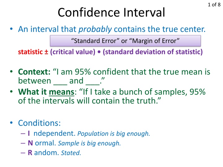
1. 1 of 8 Confidence Interval An interval that probably contains the true center. Standard Error or Margin of Error statistic (critical value) (standard deviation of statistic) Context: I am 95% confident that the true mean is between ___ and ___. What it means: If I take a bunch of samples, 95% of the intervals will contain the truth. Conditions: I ndependent. Population is big enough. N ormal. Sample is big enough. R andom. Stated.

2. Confidence Interval (one-sample mean) In December 2012, the admissions department chair of Stanford University wanted to use the IQ scores of current students as a marketing tool. He administers IQ tests to an SRS of 50 of the 6927 undergraduate students. He gets a sample mean of 112, with s=18.2. What can the director conclude about the IQ scores of Stanford undergraduates? Estimate with 95% confidence. Independence met, 6927 > 10(50). Normality met, n>30. Randomness stated. 1. Conditions. 18 2 . 112 106 . 5 96 . 04 . 1 112 96 2. Calculations. 50 117 04 . 3. Interpretation. I am 95% confident that the true mean IQ score of Stanford undergraduates is between 106.96 and 117.04.

3. 3 of 8 t-distribution If sample is big enough, you can assume s . If sample isn t big enough, you can tassume s Use t, not z. Different t-distribution for every sample size n. Specify with degrees of freedom (df) n - 1 Conditions: Independence. N 10n Normality. Look for crazy-skewed sample data. Use judgment (normal quantile plot if possible, graph #6 in StatPlot, linear=normal) Random. Usually stated.

4. 4 of 8 Mean Proportion Is n>30? Is np>10 and n(1-p)>10? YES YES NO NO Use z. Use z. You have Normality. You have Normality. Is it Normal? (quantile plot) Is it Normal? (quantile plot) YES NO YES NO You re screwed. You re screwed. Use t. Use t.

5. 1.28 1.17 1.16 1.08 0.6 1.32 1.24 0.71 0.49 1.38 1.2 0.78 0.95 2.2 1.78 1.83 1.26 1.73 1.31 1.8 1.15 0.97 1.12 EXAMPLE: Conf. interval, small sample (t) Environmentalists, government officials, and vehicle manufacturers are all interested in studying the auto exhaust emissions produced by cars. A primary pollutants in exhaust is nitrogen oxides (NOX). Here are the NOX levels (in grams per mile) for a random sample of light-duty engines of the same type. Construct and interpret a 95% confidence interval for the mean amount of NOX emitted by light-duty engines of this type. Independence is met, N>220. Normality is assumed based on the linearity of a normal quantile plot, after removing an outlier (2.2) based on the 1.5xIQR rule. Randomness stated. calculator . 1 24 . 0 164 calculator . 0 369 . 1 20 . 2 08 22 . 1 . 1 076 404 t-chart, df=21 I am 95% confident that the true mean NOX emissions by light- duty engines of this type is between 1.076 and 1.404.

6. 6 of 8 Is caffeine dependence real? Researchers at the University of Minnesota (Bernstein et. Al, 2002) studied 11 people diagnosed as being caffeine- dependent. Each subject was barred from consuming caffeine. Instead, they took capsules containing their normal caffeine intake. During a different time period, they took placebo capsules. The table below contains data on one of several tests given to the subjects. Construct and interpret a 90% confidence interval for the mean change in depression. Subject 1 2 3 4 5 6 7 8 9 10 11 Depression (caffeine) 5 5 4 3 8 5 0 0 2 11 1 Depression (placebo) 16 23 5 7 14 24 6 3 15 12 0

7. 7 of 8 Is caffeine dependence real? Subject 1 2 3 4 5 6 7 8 9 10 11 Depression (caffeine) 5 5 4 3 8 5 0 0 2 11 1 Depression (placebo) 16 23 5 7 14 24 6 3 15 12 0 Caffeine placebo -11 -17 -1 -4 -6 -19 -6 -3 -13 -1 1

8. 8 of 8 Is caffeine dependence real? Researchers studied 11 people diagnosed as being dependent on caffeine. The table below contains data on two of several tests given to the subjects. Construct and interpret a 90% confidence interval for the mean change in depression. Caffeine placebo -11 -17 -1 -4 -6 -19 -6 -3 -13 -1 1 Independence met, N>110. Normality met, with no apparent outliers and approximate linearity on a normal quantile plot. Randomness not met, not stated. 77 . 6 812 . 1 27 . 7 27 . 7 . 3 10 97 . 57 . 3 70 11 If randomness was met, I d be 90% confident that the true mean change in depression when patients take caffeine vs. placebos is between -10.97 and -3.57.