Principles of Finance: Understanding Discounting, Present Value, and Market Equilibrium
Delve into the foundational concepts of finance with topics such as discounting, present value computations, the law of one price, equilibrium, and market arbitrage. Explore how prices are determined, the relationship between demand and supply, and the factors influencing market equilibrium. Gain insights into how markets tend towards balance and the impact of operational costs on price discrepancies.

Download Presentation

Please find below an Image/Link to download the presentation.
The content on the website is provided AS IS for your information and personal use only. It may not be sold, licensed, or shared on other websites without obtaining consent from the author. Download presentation by click this link. If you encounter any issues during the download, it is possible that the publisher has removed the file from their server.
E N D
Presentation Transcript
1 P.V. VISWANATH FOR A FIRST COURSE IN FINANCE
2 The conceptual basis behind discounting and present value computations Law of One Price, Equilibrium and Arbitrage What is the relationship between prices at different locations Prices and Rates Where do we get interest rates from? Annualizing Rates How do we annualize rates?
3 In the absence of frictions, the same good will sell for the same price in two different locations. For example, if a pair of shoes trades at one location for $100, it must trade at all locations for the same $100. If goods are sold in different locations using different currencies, then The law of one price says: after conversion into a common currency, a given good will sell for the same price in each country. If $1= 0.8 ( 1=$1.25), and a bushel of wheat sells for $15, it must sell for (15)(0.8) or 12 in the UK. A simple reason why the LOP should hold is that buyers will simply go to the lower cost seller and sellers will sell to the person offering the highest price. This is part of market equilibrium. Let s first see how equilibrium works, how prices are determined in free markets.
4 At any given price for a good, there will be some number of individuals who will be willing to buy the good (demand the good). This number will increase as the price drops. The locus of these [price, demand] pairs gives us the demand schedule (or curve), D. Similarly, at any given price, there will be some number of individuals willing to sell the good (supply the good). This number will decrease as the price drops. The locus of these price, demand pairs gives us the supply schedule (or curve), S. The intersection of these two curves is the equilibrium price, P0. At this price, the quantity demanded of the good is exactly equal to the quantity supplied. Furthermore, if the price for any reason is greater than P0 (say P1), the supply will be greater than the demand; in order to sell the excess supply, suppliers will reduce the price until the price is once again P0 and the market is in equilibrium.
5 Price S Supply curve P1 P0 Demand Curve D Q1 Q0 Quantity
6 We see that markets tend towards equilibrium, in which there is a single price and, at this price, supply equals demand. There are no forces requiring prices to change unless the underlying fundamentals change. This is true if trading is costless, i.e. if there are no frictions. What sort of frictions can cause there to be trades at more than one price? Suppose there are operational costs of trading, e.g. if selling a good requires setting up a shop, or it requires tying up capital. Assume for convenience that this cost can be converted into a per unit value of $1. Then the seller will not be willing to buy at the same price as his selling price because he would then incur a loss of $1/unit. In this case, the selling price will be $1 higher than the buying prices, as you can see in the next figure.
7 Price S Supply curve Paprice buyers pay Cost of trading = $1.00 P0 Pb price sellers get Demand Curve D Q1 Q0 Quantity
8 Equilibrium will not be at a price of P0, because at that price, the demand will be Q0; however, the supply will be less than Q0 because the seller will only get a price equal to P0-1. However, at an asking price of Pa, demand will be Q1 and supply will also be exactly Q1, because the price that sellers get will be Pa-1, and the supply at that price is exactly Q1., Pa is called the ask price, the price at which a seller stands ready to sell the good. Pb is the bid price, the price at which the seller stands ready to buy the good. This is so, because if he buys it at Pb, he can turn around and cover his costs by selling it at Pa (which is equal to Pb+1).
9 Clearly, if trading costs are lower in some places, then ask prices will be lower and the difference between the bid and ask prices (the bid-ask spread) will also be lower there. If buyers also have costs of trading, the market may be segmented into several submarkets with their own prices and bid-ask spreads, but the differences will be restricted by the costs of moving from one market to another. If there are no frictions, the price will be exactly P0 in equilibrium.
10 In what follows, we will assume that there are no frictions. This is close to the situation in financial markets, where what is traded is simply a legal claim to cashflows. If there are no frictions, the price of the good would be P0 in equilibrium everywhere; that is, the law of one price holds. However, there are stronger forces than equilibrium that will ensure that the law of one price holds, viz. arbitrage. The way that arbitrage works is very simple. Suppose the price at which a good is sold were to be P1 at location 1 and P0 < P1 at location 0. Then, it would be easy to make money by buying at P0 and selling at P1. This will force the price at location 0 to rise and/or the price at location 1 to fall until both prices converge to the same price.
11 How about if there is a price P0 in market 0 and one seller increases his ask price to P1 > P0? That is, he sells at P1 and buys at P0. There is no arbitrage possibility, now, so these prices might remain for a while. Some buyers might even buy from him at the higher price P1. However, eventually, prices will converge to a single price because as all buyers learn about the lower price, they will stop patronizing the higher-price seller. This is the equilibrium that we spoke about earlier. In financial markets, transactions costs are small enough that for many purposes, we can ignore them. This means that we can act as if there is a single price at which financial goods (assets) are traded. Arbitrage (aided by equilibrium) will ensure that there is a single price for every asset.
12 A financial asset is an asset that generates future cashflows. In finance, we assume that these cashflows are the only relevant characteristic of an asset. Combined with the law of one price, this assumption allows for some powerful pricing techniques. Assume for now that cashflows are riskless. Denote by pt, the price today (t=0) of an asset that pays of exactly $1 at time t and zero at all other times; let s call these primary assets. Thus p20 will be the price at t=0 of an asset that will have a cashflow of $1 at t=20 and $0 at all other times. The price of this asset at t=19 and at all other times will be positive, but less than one. In particular, its price p20 at t=0 will also be positive, but less than one. Keep in mind that the t=0 price of a future cashflow is another way of saying present value of the future cashflow.
13 Arbitrage refers to The process by which investors take advantage of price discrepancies The process by which investors choose assets best fit their investment goals The process by which supply and demand equilibrate.
14 Then the number of primary assets that need to be priced is exactly the number of time periods. The prices of these primary assets are assumed to be determined in financial markets and are taken to be known. We will now consider how primary asset prices can be used to price financial assets, other than primary assets. Denote by ctj, t=1, ,T, the amount of the cashflow that asset jwill pay off at time t=1, ,T. Then the price of the asset j will be exactly Pj = t=1,..,Tctjpt In other words, the price of the asset is the sum of the present values of each future cashflow.
15 If the primary assets are traded in frictionless markets, then the law of one price will ensure that they all sell at the same price. But what about other assets, such as asset j with cashflows {ctj, t=1, ,T}, that are not primary assets? Even if markets for these other assets are illiquid, the law of one price will hold for them as well! The reason is that any such asset can be created as a portfolio of the primary assets. And if these assets are not even traded, we can use the value of the equivalent portfolio of primary assets to generate the market value they would have if they were traded.
16 Suppose we have non-traded financial assets that promise riskfree cashflows of $40 every year for the next 3 years. We have an opportunity to buy this asset. But how much should we bid for this asset? This asset is equivalent to a portfolio consisting of 40 units of primary asset 1, 40 units of primary asset 2 and 40 units of primary asset 3. Thus, according to the LOP, this non-traded assets if it were to trade would sell for exactly 40(p1) + 40(p2) + 40(p3), where pi is the price of primary asset i. This is what we would bid for this asset.
17 Suppose we have a capital budgeting project, an investment in a factory that requires an investment of $10m. today. Our marketing managers and our production managers have worked out the optimal production and marketing strategies. They believe this factory will generate after-tax risk-free cashflows of $5m in 1 year, $3m in 2 years and $4m in 3 years. At that point, all assets will be fully depreciated. This project is equivalent to a portfolio of 5m units of primary asset 1 (each one paying $1 at t=1 and nothing at any other time), 3m units of primary asset 2 and 4m assets of primary asset 3. Once we have the prices of these primary assets, p1, p2 and p3, we can value the cashflows from our factory at 5m(p1) + 3m(p2) + 4m(p3) because a financial security promising these same cashflows would sell for exactly this amount. If this valuation > than $10m, the investment is worthwhile.
18 Where do we get the primary asset prices? We have to go to the market and observe prices of complex traded financial securities. Suppose we have three assets, A, B and C. They have the following cash flows and prices: Asset Price today cashflow A 50.63 B 26.00 C 71.15 t=1 t=2 cashflow t=3 cashflow 20 20 20 10 20 55 20 5
19 We first create the equivalent portfolios of primary assets as we did before. Then, using our previous notation of pi is the price of primary asset i , we can write these equations: pA = 50.63 = 20(p1) + 20(p2) + 20(p3) pB = 26.00 = 10(p1) + 20(p2) pC = 71.15 = 55(p1) + 20(p2) + 5(p3) These simultaneous equations can be solved easily to find that p1 = 0.917, p2 = 0.842 and p3 = 0.772. Now we go back to our capital budgeting problem and our problem of valuing non-traded assets.
20 The value of the non-traded asset we had worked out to be 40(p1) + 40(p2) + 40(p3). Given the primary asset prices, we can computed its price as 40(0.92) + 40(0.84) + 40(0.77) = 101.25. The present value of the factory investment we know is 5m(p1) + 3m(p2) + 4m(p3). Substituting, we get 5m(0.92) + 3m(0.84) + 4m(0.77) = $10.20093m. Hence investing $10m in this factory is worthwhile, because we could sell the cashflows from this factory to get an immediate price of $10.20093m and make an immediate profit of $200,930. Even if for some reason, we choose not to sell the right to these cashflows, our wealth immediately increases by the amount of $200,930.
21 Asset j {with cashflows ctj, t=1, ,n} can be synthesized by putting c1j units of primary asset 1, c2j units of primary asset 2, etc. and so on into a synthetic portfolio. This means that the original asset j must trade at the price Pj. If it traded at a higher price, people would create the synthetic portfolio for a cost of Pj and sell it in the market for asset j at the higher price and thus make money. If it traded at a lower price, people would buy asset j and using it as collateral, create the corresponding primary assets and sell them for a collective higher price of Pj and thus make money.
22 Suppose there were an asset X that promised payment of $100 at time 1 and $200 at time 2. This could be synthesized by taking 100 units of primary asset 1 and 200 units of primary asset 2. If p1 were 0.9 and p2 were 0.82, then asset X would have to sell for 0.9(100) + 0.82(200) = $254. Why? If the price of asset X were higher (say $260), people would create new units of asset X by using the synthetic strategy described above (for $254) and sell them for $260, making $6 on every trade. If the price of asset X were lower (say $250), people would buy asset X for $250 and sell 100 primary asset 1 claims and 200 primary asset 2 claims for $254. They would make $4 on each trade and would be able to pay off the claims made by the purchasers of these claims in periods 1 and 2 by using the cashflows from asset X. This is how the pricing of ETFs stay close to the value of the underlying securities that are bundled in each ETF.
23 When recovering primary asset prices, do we need to pick a particular set of complex asset prices? Will we get different values for the primary asset prices? The answer is that as long as the LOP holds, you can pick any set of complex assets. Suppose we used assets the prices pA and pB and get one set of primary asset prices, p1(AB) and p2(AB). Suppose using the prices of assets pC and pD gives us different values of p1(CD) and p2(CD). This means that if we valued asset C using p1(AB) and p2(AB), we would get a different value p . So let s assume that p < pC. Then we can use assets A and B to create a portfolio that has the same cashflows as asset C at a cost of p . We can then sell it at pC because this synthetic asset C is identical to the real asset C. This would give us an arbitrage profit! If the Law of One Price holds, this should not be possible. In other words, we will get the same primary asset prices, no matter which complex assets we use to recover the primary asset prices.
24 When we talk of pricing primary assets or other financial assets that pay off in future periods, we are talking about their price in t=0 dollars, i.e. in current dollars. As mentioned before, this is precisely what we mean by present value. So as we go forward with our discussion, pricing financial assets is equivalent to obtaining the present value of the future cashflows that they represent. The key to the pricing rules to be described below is the pricing of primary assets. Our next goal is to represent the pricing of these primary assets using discount rates. Let s start by understanding these primary assets better.
25 Consider a primary asset paying exactly $1 at time t=1 & zero at all other times. In our notation, the price of this asset is p1. What is this asset? This is the right to a dollar, but one that you will only get (and be able to spend) one period hence (t=1); we could call this a t=1 dollar; similarly we could have t=2 dollars, etc. A t=0 dollar, we will simply call a dollar or a current dollar. Assume that the price of a t=1 dollar is $0.90, the price of a t=2 dollar is $0.7831 and the price of a t=3 dollar is $0.675, where these prices are denominated in current dollars, i.e. dollars that you can spend immediately. This is just as like saying that the price of a book is $10, the price of a subway token is $2 and the price of a cup of Starbucks coffee is $3.50.
26 The following is a correct example of a primary asset: An asset that pays $1 each period for the next 10 periods. Yes No
27 We are used to hearing that the price of a cup of coffee is a certain number of dollars, say $3.50. Let us consider another way to denote this same price. Suppose Starbucks required everybody to play the following game in order to figure out the price of its offering. Suppose they took the actual dollar price of a coffee multiplied it by 2 and added 3 to it and called it java units (J). A cup of coffee that normally cost $3.5 would be listed as costing 10J. Then if we saw a cappuccino listed at 13J, we would simply subtract 3 to get 10, then divide by 2 to get a price of $5. It would be a little weird, but nothing substantive would change.
28 Just as we expressed the price of a cup of coffee in two different ways, a dollar price and a Java price, let s represent the price of a future dollar in two different ways. One way is simply the dollar price. Thus, p1, the price of a t=1 dollar is $0.90. Now for the other method. If we buy a t=1 dollar and hold it for one period, it becomes a current dollar and would be worth $1. Thinking of this as an investment strategy, the one period return on a t=1 dollar is 1/0.9 -1 or 11.11%. We can describe p1 fully either by giving its numerical value of $0.9 or by stating that the 1-period rate of return on a t=1 dollar is 11.11%, since both are equivalent. Call this the r-price or r1. We saw how to recover a dollar price from a J-price. How do we get a dollar price from a r-price? Since 1/0.9 -1 or 11.11%, i.e. p1, 1/ p1 1 = r1 i.e. p1 = 1/(1+r1), i.e. 0.9 = 1/(1+0.11) = 1/1.11 This process of recovering a dollar price from an r-price (or discount rate) is called discounting.
29 If the price today of a security paying $1 at time 1 is 0.95 in current dollars, what is the r-price (i.e the discount rate)? A. 5.26% B. 5% C. 4.76%
30 What about the price of a t=2 dollar, which we said was $0.7831? Once again, the price of this t=2 dollar would be $1 at t=2 (in current dollars, since at t=2, the t=2 dollar itself becomes a current dollar). We could compute the gross return on this investment, in the same way, as 1/0.7831 = 1.277 or a return of 27.70%. But this is a return over two periods, and we cannot compare it directly to the 11.11% that we computed earlier. Right now, we really don t have any reason to make such a comparison, but when we start talking about the yield curve, we may want to make such comparison. So let s express the two-period return in a form that is comparable to the one-period return. The question is: how? The solution to this problem is to annualize the two-period return.
31 We computed the two-period return on buying a t=2 dollar at 27.70%. Let s define the one-period period return on any two-period investment as that return, which earned sequentially over the two periods gives us our two-period return. Suppose this posited one-period return is r2%; that is, the return from holding this t=2 dollar from now until t=1 is r2 %. Then, every dollar invested in this specialized investment could be sold at $(1+ r2) at t=1. The return on this t=2 dollar if held from t=1 to t=2 is also r2 %, as assumed. Hence the t=1 $(1+ r2) value of our original outlay of one t=0 dollar becomes $(1+ r2)(1+ r2) or (1+ r2)2 at t=2. The gross return on this investment is 1/0.7831 = 1.277 = 1 plus the two period return, i.e. 1/p2 = (1+ r2)2. Hence p2 = 1/(1+ r2)2. Conversely, p2 = [1/(1+ r2)]2gives us p2 = 1/(1+ r2) or r2= p2-1 .
32 In our example, we already know from our return computation, that this is exactly 1.277 (that is 1 plus the 27.7%). Hence we equate (1+r)2 to 1.277 and solve for r to get the one-period return. This involves simply taking the square-root of 1.277, which is 13%. Of course, we won t get exactly 13% in each of the two periods. The 13% rate is, rather, a sort of average return over the two periods, that results in a 27.7% over the two years.
33 We can do the same thing with the price of a t=3 dollar, as well. Remember that the way we got 27.7%, the two-period return on the t=2 dollar ,was by computing 1/0.7831 = 1.277. Similarly, to get the return on the t=3 dollar investment we simply take $0.675, the price of a t=3 dollar and also convert it to a rate of return. In this case, we take the cube root of (1/0.675) and subtract 1, which gives us 14%. In these examples, we took a return earned over more than one year and expressed it in terms of an annualized return. Later we will learn about how to take a return earned over less than one year and express it in terms of an annualized return.
34 If p3 = .72, the corresponding r-rate or discount rate is A.12.5% B. 11.57% C. 17.85% D. 38.89%
35 The purpose of this exercise is to be able to use r-unit prices or discount rates to price financial assets instead of current dollar prices. The two methods are equivalent. Suppose we have a security that gives us the right to obtain $20 at t=1. What is its price today? Method 1: We know that the price today of $1 at t=1 is 0.90. Hence the price of the security is 20(0.90) = $18. Method 2: If we know the r-unit price (or the discount rate), we can convert the r-unit price into a current dollar price by using the formula p1 = 1/(1+r1). In our example, if we didn t know the current dollar price, but we did know the r-unit price of 11%, we can recover the current dollar price thus: p1 = (1/1.11) = 0.90. Hence, instead of computing 20(0.90), we can also compute 20(1/1.11) or 20/1.11 to get the same answer of $18.
36 Suppose we have a security that gives us the right to obtain $20 at t=2. What is its price today? Method 1: We know that the price today of $1 at t=2 is 0.7831. Hence the price of the security is 20(0.7831) = $15.662. Method 2: If we know the r-unit price (or the discount rate), we can convert the r-unit price into a current dollar price by using the formula p2 = 1/(1+ r2)2. In our example, if we didn t know the current dollar price, but we did know the r-unit price of 13%, we can recover the current dollar price thus: p2 = (1/1.13)2 = 0.7831. Hence, instead of computing 20(0.7831), we can also compute 20(1/1.13)2 or 20/(1/1.13)2to get the same answer of $15.662.
37 If we have a security paying $c at time 1, (which is equivalent to having c primary securities paying $1 at time 1), and we know that its d-unit price is r, then its current dollar price is c/(1+r1). If we have a security paying $c at time 2, (which is equivalent to having c primary securities paying $1 at time 2), its price today is c/(1+rt)2. If we have a security paying $c at time t, (which is equivalent to having c primary securities paying $1 at time t), its price today is c/(1+rt)t. The process of computing the price of a future cashflow by dividing it by (1+rt)t is called discounting.
38 The whole point of the exercise is the presumption that it might be easier to locate discount rates or d-unit prices than current dollar prices for primary assets. So where do we get these discount rates? Remember that the discount rates, which are just the rates of return are nothing more than transformations of the current dollar prices for the primary assets. If so, then we have to make sure that the discount rates that we use to price (get the present value of) assets must be the rates of return on the right assets. Thus, if we are dealing with primary assets that are risk-free, then we need the rates of return on risk-free assets. In this case, we can use the rates of return on the appropriate Treasury securities. If our primary assets are risky, on the other hand, then we have to make sure that we get the rates of return on assets that have similar risk.
39 You are thinking of buying an annuity sold by a private company which promises to pay $100 each year for the next 10 years. In order to come up with a valuation for the annuity, you look for a discount rate to discount the promised cashflows. The correct discount rate is: The 10-year T-bond rate The market rate of return on securities that are comparable to this annuity. The risk-free rate
40 To summarize, if we have an asset with cashflows {ctj, t=1, ,T}, its price can be computed as Pj = t=1,..,Tctj/(1+rt)t, where the discount rates rt represent the rates of return on assets with the same risk as the associated cashflow ctj. As we saw before, this depends upon the no-arbitrage rule, which, in turn, depended upon the existence of a liquid market for primary securities. What if the primary securities were not traded? In that case, we could still imagine prices pt for the primary securities underlying the prices of other traded complex non- primary financial assets. Economists have come up with techniques to recover prices/discount rates for primary securities from the prices of the traded financial assets.
41 Even though there are techniques to recover prices/discount rates for primary assets, it is still true, however, that we must have enough assets that are traded to be able to reconstruct underlying rates with any degree of precision. For riskless cashflows, there is no problem because we have a liquid market for Treasury assets. For risky primary assets that we want to price, however, we may not find traded assets with precisely the same kind of riskiness. What do we do in this case? In practice, what we want to price most often are not primary assets, but portfolios of primary assets. For example, in capital budgeting, which we will discuss in a later module, we may be considering a project for which we have forecasted future cashflows. Is it worth investing in? Or not? Here, we use what is known as the NPV rule. Let s look at this further.
42 If a manager had the opportunity to invest in a project that generated cashflows {ctj, t=1, ,T}. We would like to determine Pj, its price in the open market. As long as he could obtain the right to invest in that project for less than Pj , the project would be worthwhile. The initial required investment, c0 in a project is the cost of the right to invest in the project. Hence the manager should invest in the project if Pj = t=1,..,Tctj/(1+rt)t > c0; i.e. if NPV = t=1,..,Tctj/(1+rt)t - c0 >0. This is called the NPV rule.
43 How can we extract the prices of riskless primary securities from the prices of complex, riskless securities? This can be done by using Treasury securities. Here s an example: on Feb. 21, 2008, a 6-month Treasury bill (or T-bill) issued sold for 98.968667 of face value. A T-bill is a promise to pay money 6 months in the future. With the given price then, a buyer would get a 1.042% return for those 6 months. This is often annualized by multiplying by 2 to get an APR (called a bond-equivalent yield) of 2.084%. Wherever Treasury bills exist for the dates we are interested in, we can compute the discount rates directly from their prices, because these are primary securities. However such primary securities (T-bills) don t exist for longer maturities. For these dates, we use Treasury bonds and Treasury notes.
44 For example, on Feb. 29th 2008, the Treasury issued a 2-year 2% note with a maturity date of February 28, 2010 with a face value of $1000, which was sold at auction. The price paid by the lowest bidder was 99.912254% of face value. This means that the buyer of this bond would get every six months 1% (half of 2%) of the face value, which in this case works out to $10. In addition, on Feb. 28, 2010, the buyer would get $1000. Such securities of longer duration are called bonds. These are examples of the complex financial securities from which we can derive the discount rates of primary securities.
45 Suppose not all primary assets are traded. In this case, we can estimate the implicit prices or interest rates as follows: Suppose we have K different traded financial assets generating cashflows, {ctj, t=1, ,T, j=1, ,K}. We have the prices of these K assets call them Pk. Then we have the K equations Pk = t=1,..,Tctkpt. If K=T, then we have a system of equations that we can solve for the primary asset prices pt, t=1, ,T and then work back to get the interest rates, rt, t=1, ,T. If K < T, then there are many solutions to this system of equations. In that case, some assumptions are made about how rt varies as t changes. For example, presumably there will be some continuity r2 will probably be close to r1 etc.
46 But how do we get the discount rates rt that are associated with the risky cashflows, ctj? What we need to do first is to define cashflow risk in a precise sense. Once this is done, economists have ways of recovering the underlying prices of the risky primary assets. One practical way is to give up the notion of a primary asset and work directly with the actual complex financial assets that we want to price, such as a capital budgeting project or a private business. We then come up with a loose measure of risk, such as a P/E ratio. We then find other traded securities that have similar P/E ratios. The average return on these comparable securities could then be used as the discount rate to price our asset of interest.
47 Economists also use Asset Pricing Models to value securities when cashflows are risky. First they make assumptions about individual behavior and the investment environment to come up with a measure of risk. For example, if we accept the assumptions of the CAPM, the beta is a good measure of risk of a particular cashflow. They then look at how this measure of risk would be related to expected return in equilibrium if people behaved according to the assumptions of the model. This allows them to associate an expected rate of return with each cashflow. Then, as before, expected cashflows are discounted using this expected rate of return.