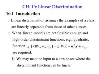
Linear SVMs for Binary Classification
Support Vector Machines (SVMs) with linear kernels are powerful tools for binary classification tasks. They aim to find a separating hyperplane that maximizes the margin between classes, focusing on support vectors closest to the decision boundary. The formulation involves optimizing a quadratic problem to find the hyperplane parameters w and b that best separate the data points. Linear SVMs emphasize maximizing the margin and are effective in scenarios where data points are linearly separable.
Download Presentation
Please find below an Image/Link to download the presentation.
The content on the website is provided AS IS for your information and personal use only. It may not be sold, licensed, or shared on other websites without obtaining consent from the author. Download presentation by click this link. If you encounter any issues during the download, it is possible that the publisher has removed the file from their server.

Presentation Transcript
Support Vector Machines Kernels based on notes by Andrew Ng and Others
Problem definition: -We are given a set of n points (vectors) : such that is a vector of length m , and each belong to one of two classes we label them by +1 and -1 . -So our training set is: ( , ),( , ),....( , ) n n x y x y x y , { 1, 1} i i i x R y + , ,....... x x x ix 1 2 n So the decision function will be ( ) f x sign w x b = + ( ) 1 1 2 2 m - We want to find a separating hyperplane that separates these points into the two classes. The positives (class +1 ) and The negatives (class -1 ). (Assuming that they are linearly separable) w x b + = 0
Machine Learning Group Linear Separators Which of the linear separators is optimal? 3 University of Texas at Austin
Machine Learning Group Classification Margin + T w x b Distance from example xito the separator is Examples closest to the hyperplane are support vectors. Margin of the separator is the distance between support vectors. = i r w r 4 University of Texas at Austin
Machine Learning Group Maximum Margin Classification Maximizing the margin is good according to intuition and PAC theory. Implies that only support vectors matter; other training examples are ignorable. 5 University of Texas at Austin
Machine Learning Group Linear SVM Mathematically Let training set {(xi, yi)}i=1..n, xi Rd, yi {-1, 1} be separated by a hyperplane with margin . Then for each training example (xi, yi): wTxi+ b - /2 if yi= -1 wTxi+ b /2 yi(wTxi+ b) /2 if yi= 1 For every support vector xsthe above inequality is an equality. After rescaling w and b by /2 in the equality, we obtain that distance between each xs and the hyperplane is + T w x y ( ) 1 b = = s s r w w Then the margin can be expressed through (rescaled) w and b as: 2 2 = = r w 6 University of Texas at Austin
Machine Learning Group Linear SVMs Mathematically (cont.) Then we can formulate the quadratic optimization problem: Find w and b such that 2 = is maximized w and for all (xi, yi), i=1..n : yi(wTxi+ b) 1 Which can be reformulated as: Find w and b such that (w) = ||w||2=wTw is minimized and for all (xi, yi), i=1..n : yi(wTxi+ b) 1 7 University of Texas at Austin
SVM : Linear separable case. The optimization problem: -Our optimization problem so far: 1 2 I do remember the Lagrange Multipliers from Calculus! w minimize 2 + ) 1 T s.t. w x ( y b i i -We will solve this problem by introducing Lagrange multipliers associated with the constrains: i 1 minimize ( , , ) 2 . i st n 2 = + ) 1) ( ( L w b w y x w b p i i i = 1 i 0
constrained optimization on convex set X , given convex functions f , g1, g2, ...., gk, h1,h2, ...., hm the problem minimize f (w) subject to gi(w) 0 ,for all i hj(w) = 0 ,for all j set. If f is strict convex the solution has as its solution a convex is unique (if exists) we functions f , g1, g2, ...., gk, h1, h2, ...., hm like convexity, differentiability etc.T hat will still not be enough though.... will assume all the good things one can imagine about 14
equality constraints only minimize f (w) subject to hj(w) = 0 ,for all j define the lagrangian function ! L(w, ) = f (w) + jhj(w) j L agrange t heorem nec[essary] and suff[icient] conditions for a point " existence of "such that wL( "w, ) = 0 ; w to be an optimum (ie a solution for the problem above) are the jL(w, ) = " " " 0 15
inequality constraints minimize f (w) subject to gi(w) 0 ,for all i hj(w) = 0 ,for all j we can rewrite every inequality constraint hj(x) = 0 as two inequalities hj(w) 0 and hj(w) 0. so the problem becomes minimize f (w) subject to gi(w) 0 ,for all i 18
Karush Kuhn Tucker theorem minimize f (w) subject to gi(w) 0 ,for all i were gi are qualifi ed const raint s define the lagrangian function ! L(w, ) = f (w) + igi(w) i K K T t heorem nec and suff conditions for a point w to be a solution for the optimization problem are the existence of " such that wL( "w, " ) = 0 ; #igi(w) = gi( "w) 0 ; #i " " 0 0 19
KKT - sufficiency w, " ) satisfies KKT conditions $k " " w) = 0; #i 0 Assume ( " wL( " w, " ) = wf (w) + L w, ) = gi(w) 0 #igi( " w) = 0 #i wgi( " i= 1 ( " " i T hen f (w) f ( " $ki= 1 #i( wgi( "w))T(w w) $k w) ( wf (w))T(w w) = " " w #i(gi(w) gi( " )) = " i= 1 $k i= 1 #igi(w) 0 so w is solution " 20
saddle point minimize f (w) subject to gi(w) 0 ,for all i and the lagrangian function ! L(w, ) = f (w) + igi(w) i ( "w, " ) with #i 0 is saddle point if (w, ), i 0 w, ) L(w, " ) L(w, " ) L( " " 21
200 0 ! 200 ! 400 ! 600 ! 800 ! 1000 ! 10 ! 1200 ! 5 ! 1400 0 0 2 5 13 4 6 8 10 10 w alpha
saddle point - sufficiency minimize f (w) subject to gi(w) 0 ,for all i $ lagrangian function L(w, ) = f (w) + igi(w) w, " ) is saddle point " ) i ( " (w, ), i 0 : L( " , ) L( " , " ) L(w, w w then 1.w is solution to optimization problem 2. #igi(w) = 0 for all i " " 23
saddle point - necessity minimize f (w) subject to gi(w) 0 ,for all i were gi are qualifi ed const raint s $ lagrangian function L(w, ) = f (w) + igi(w) w is solution to optimization problem i " then w, " ) is saddle point " ) w " 0 such that ( " (w, ), i 0 : L( " , ) L( " , " ) L(w, w 24
constraint qualifications minimize f (w) subject to gi(w) 0 , for all i let be the feasible region = { w|gi(w) 0 i} then the following additional conditions for functions gi are connected (i) (ii) and (iii) (i) : (i) there exists w such that gi(w) 0 i (ii) for all nonzero [0, 1)k w such that igi(w) = 0 i (iii) the feasible region contains at least two distinct elements, and w such that all gi are are strictly convex at w w.r.t. 25
Machine Learning Group Theoretical Justification for Maximum Margins Vapnik has proved the following: The class of optimal linear separators has VC dimension h bounded from above as , min 2 2 D + 1 h m 0 where is the margin, D is the diameter of the smallest sphere that can enclose all of the training examples, and m0is the dimensionality. Intuitively, this implies that regardless of dimensionality m0 we can minimize the VC dimension by maximizing the margin . Thus, complexity of the classifier is kept small regardless of dimensionality. 26 University of Texas at Austin
Machine Learning Group Soft Margin Classification What if the training set is not linearly separable? Slack variables ican be added to allow misclassification of difficult or noisy examples, resulting margin called soft. i i 27 University of Texas at Austin
Machine Learning Group Soft Margin Classification Mathematically The old formulation: Find w and b such that (w) =wTw is minimized and for all (xi,yi), i=1..n : yi(wTxi+ b) 1 Modified formulation incorporates slack variables: Find w and b such that (w) =wTw + C i is minimized and for all (xi,yi), i=1..n : yi(wTxi+ b) 1 i,, i 0 Parameter C can be viewed as a way to control overfitting: it trades off the relative importance of maximizing the margin and fitting the training data. 28 University of Texas at Austin
Machine Learning Group Soft Margin Classification Solution Dual problem is identical to separable case (would not be identical if the 2- norm penalty for slack variables C i2was used in primal objective, we would need additional Lagrange multipliers for slack variables): Find 1 Nsuch that Q( ) = i- i jyiyjxiTxjis maximized and (1) iyi= 0 (2) 0 i C for all i Again, xiwith non-zero iwill be support vectors. Solution to the dual problem is: Again, we don t need to compute w explicitly for classification: w = iyixi b= yk(1- k) - iyixiTxk for any k s.t. k>0 f(x) = iyixiTx + b 29 University of Texas at Austin
Machine Learning Group Non-linear SVMs Datasets that are linearly separable with some noise work out great: x 0 But what are we going to do if the dataset is just too hard? x 0 How about mapping data to a higher-dimensional space: x2 x 0 31 University of Texas at Austin
Machine Learning Group Non-linear SVMs: Feature spaces General idea: the original feature space can always be mapped to some higher-dimensional feature space where the training set is separable: : x (x) 32 University of Texas at Austin
What Functions are Kernels? For some functions K(xi,xj) checking that K(xi,xj)= (xi)T (xj) can be cumbersome. Mercer s theorem: Every semi-positive definite symmetric function is a kernel Semi-positive definite symmetric functions correspond to a semi-positive definite symmetric Gram matrix: K(x1,x1) K(x1,x2) K(x1,x3) K(x1,xN) K(x2,x1) K(x2,x2) K(x2,x3) K(x2,xN) K= K(xN,x1) K(xN,x2) K(xN,x3) K(xN,xN) 35
Positive Definite Matrices A square matrix A is positive definite if xTAx>0 for all nonzero column vectors x. It is negative definite if xTAx < 0 for all nonzero x. It is positive semi-definite if xTAx 0. And negative semi-definite if xTAx 0 for all x. 36
SVM For Multi-class classification: (more than two classes) There are two basic approaches to solve q-class problems ( ) with SVMs ([10],[11]): 1- One vs. Others: works by constructing a regular SVM separates that class from all the other classes (class i positive and not i negative). Then we check the output of each of the q SVM classifiers for our input and choose the class i that its corresponding SVM has the maximum output. 2-Pairwise (one vs one): We construct Regular SVM for each pair of classes (so we construct q(q-1)/2 SVMs). Then we use max-wins voting strategy: we test each SVM on the input and each time an SVM chooses a certain class we add vote to that class. Then we choose the class with highest number of votes. q 2 i for each class i that = + t ( ( ) g x ) w x b
Interactive media and animations SVM Applets http://www.csie.ntu.edu.tw/~cjlin/libsvm/ http://svm.dcs.rhbnc.ac.uk/pagesnew/GPat.shtml http://www.smartlab.dibe.unige.it/Files/sw/Applet%20SVM/svmapplet.html http://www.eee.metu.edu.tr/~alatan/Courses/Demo/AppletSVM.html http://www.dsl-lab.org/svm_tutorial/demo.html(requires Java 3D) Animations Support Vector Machines: http://www.cs.ust.hk/irproj/Regularization%20Path/svmKernelpath/2moons.avi http://www.cs.ust.hk/irproj/Regularization%20Path/svmKernelpath/2Gauss.avih ttp://www.youtube.com/watch?v=3liCbRZPrZA Support Vector Regression: http://www.cs.ust.hk/irproj/Regularization%20Path/movie/ga0.5lam1.avi
SVM Implementations LibSVM SVMLight Weka Scikit-learn Python Others