Understanding Statistics for Particle Physics in Benasque TAE 2022
Explore the world of statistics for particle physics through lectures at the Benasque TAE 2022 event. Dive into topics like probability, hypothesis tests, machine learning, and more. Get insights into experimental sensitivity and systematic uncertainties to enhance your understanding of data analysis in physics.

Download Presentation

Please find below an Image/Link to download the presentation.
The content on the website is provided AS IS for your information and personal use only. It may not be sold, licensed, or shared on other websites without obtaining consent from the author. Download presentation by click this link. If you encounter any issues during the download, it is possible that the publisher has removed the file from their server.
E N D
Presentation Transcript
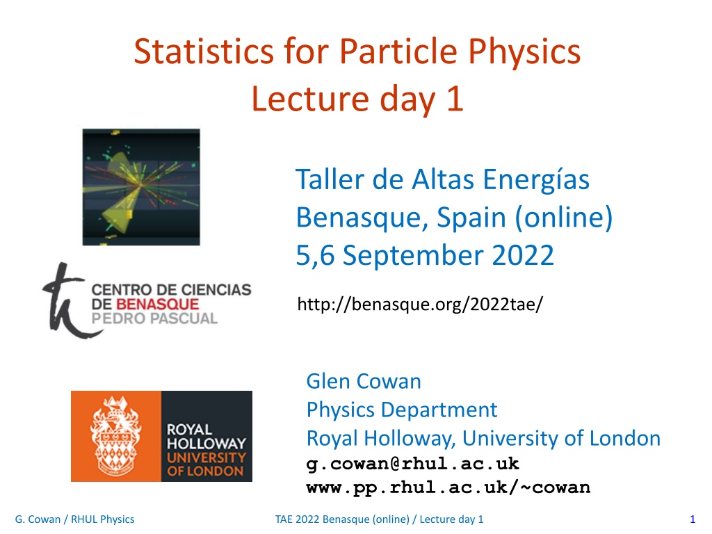
Statistics for Particle Physics Lecture day 1 Taller de Altas Energ as Benasque, Spain (online) 5,6 September 2022 http://benasque.org/2022tae/ Glen Cowan Physics Department Royal Holloway, University of London g.cowan@rhul.ac.uk www.pp.rhul.ac.uk/~cowan G. Cowan / RHUL Physics TAE 2022 Benasque (online) / Lecture day 1 1
Outline Monday 9-11 : Tuesday 9-11 : Tuesday 15:30: Introduction Probability Hypothesis tests Machine Learning Parameter estimation Confidence limits Systematic uncertainties Experimental sensitivity Tutorial on parameter estimation Almost everything is a subset of the University of London course: http://www.pp.rhul.ac.uk/~cowan/stat_course.html G. Cowan / RHUL Physics TAE 2022 Benasque (online) / Lecture day 1 2
Some statistics books, papers, etc. G. Cowan, Statistical Data Analysis, Clarendon, Oxford, 1998 R.J. Barlow, Statistics: A Guide to the Use of Statistical Methods in the Physical Sciences, Wiley, 1989 Ilya Narsky and Frank C. Porter, Statistical Analysis Techniques in Particle Physics, Wiley, 2014. Luca Lista, Statistical Methods for Data Analysis in Particle Physics, Springer, 2017. L. Lyons, Statistics for Nuclear and Particle Physics, CUP, 1986 F. James., Statistical and Computational Methods in Experimental Physics, 2nd ed., World Scientific, 2006 S. Brandt, Statistical and Computational Methods in Data Analysis, Springer, New York, 1998. R.L. Workman et al. (Particle Data Group), Prog. Theor. Exp. Phys. 083C01 (2022); pdg.lbl.gov sections on probability, statistics, MC. G. Cowan / RHUL Physics TAE 2022 Benasque (online) / Lecture day 1 3
Theory Statistics Experiment Theory (model, hypothesis): Experiment (observation): + response of measurement apparatus = model prediction data Uncertainty enters on many levels quantify with probability G. Cowan / RHUL Physics TAE 2022 Benasque (online) / Lecture day 1 4
A quick review of probability Frequentist (A = outcome of repeatable observation) Subjective (A = hypothesis) Conditional probability: E.g. rolling a die, outcome n = 1,2,...,6: A and B are independent iff: I.e. if A, B independent, then G. Cowan / RHUL Physics TAE 2022 Benasque (online) / Lecture day 1 5
Bayes theorem Use definition of conditional probability and (Bayes theorem) B If set of all outcomes S = iAi with Ai disjoint, then law of total probability for P(B) says S Ai B Ai so that Bayes theorem becomes Bayes theorem holds regardless of how probability is interpreted (frequency, degree of belief...). G. Cowan / RHUL Physics TAE 2022 Benasque (online) / Lecture day 1 6
Frequentist Statistics general philosophy In frequentist statistics, probabilities are associated only with the data, i.e., outcomes of repeatable observations (shorthand: x). Probability = limiting frequency Probabilities such as P (string theory is true), P (0.117 < s < 0.119), P (Biden wins in 2024), etc. are either 0 or 1, but we don t know which. The tools of frequentist statistics tell us what to expect, under the assumption of certain probabilities, about hypothetical repeated observations. Preferred theories (models, hypotheses, ...) are those that predict a high probability for data like the data observed. G. Cowan / RHUL Physics TAE 2022 Benasque (online) / Lecture day 1 7
Bayesian Statistics general philosophy In Bayesian statistics, use subjective probability for hypotheses: probability of the data assuming hypothesis H(the likelihood) prior probability, i.e., before seeing the data posterior probability, i.e., after seeing the data normalization involves sum over all possible hypotheses Bayes theorem has an if-then character: If your prior probabilities were (H), then it says how these probabilities should change in the light of the data. No general prescription for priors (subjective!) G. Cowan / RHUL Physics TAE 2022 Benasque (online) / Lecture day 1 8
Hypothesis, likelihood Suppose the entire result of an experiment (set of measurements) is a collection of numbers x. A (simple) hypothesis is a rule that assigns a probability to each possible data outcome: = the likelihood of H Often we deal with a family of hypotheses labeled by one or more undetermined parameters (a composite hypothesis): = the likelihood function Note: 1) For the likelihood we treat the data x as fixed. 2) The likelihood function L( ) is not a pdf for . G. Cowan / RHUL Physics TAE 2022 Benasque (online) / Lecture day 1 9
Frequentist hypothesis tests Suppose a measurement produces data x; consider a hypothesis H0 we want to test and alternative H1 H0, H1 specify probability for x: P(x|H0), P(x|H1) A test of H0is defined by specifying a critical region w of the data space such that there is no more than some (small) probability , assuming H0 is correct, to observe the data there, i.e., P(x w | H0) data space Need inequality if data are discrete. is called the size or significance level of the test. If x is observed in the critical region, reject H0. critical region w G. Cowan / RHUL Physics TAE 2022 Benasque (online) / Lecture day 1 10
Definition of a test (2) But in general there are an infinite number of possible critical regions that give the same size . Use the alternative hypothesisH1 to motivate where to place the critical region. Roughly speaking, place the critical region where there is a low probability ( ) to be found ifH0 is true, but high if H1 is true: G. Cowan / RHUL Physics TAE 2022 Benasque (online) / Lecture day 1 11
Classification viewed as a statistical test Suppose events come in two possible types: s (signal) and b (background) For each event, test hypothesis that it is background, i.e., H0 = b. Carry out test on many events, each is either of type s or b, i.e., here the hypothesis is the true class label , which varies randomly from event to event, so we can assign to it a frequentist probability. Select events for which where H0 is rejected as candidate events of type s . Equivalent Particle Physics terminology: background efficiency signal efficiency G. Cowan / RHUL Physics TAE 2022 Benasque (online) / Lecture day 1 12
Example of a test for classification Suppose we can measure for each event a quantity x, where with 0 x 1. For each event in a mixture of signal (s) and background (b) test H0 : event is of type b using a critical region W of the form: W = {x : x xc}, where xcis a constant that we choose to give a test with the desired size . G. Cowan / RHUL Physics TAE 2022 Benasque (online) / Lecture day 1 13
Classification example (2) Suppose we want = 10 4. Require: and therefore For this test (i.e. this critical region W), the power with respect to the signal hypothesis (s) is Note: the optimal size and power is a separate question that will depend on goals of the subsequent analysis. G. Cowan / RHUL Physics TAE 2022 Benasque (online) / Lecture day 1 14
Classification example (3) Suppose that the prior probabilities for an event to be of type s or b are: s = 0.001 b = 0.999 The purity of the selected signal sample (events where b hypothesis rejected) is found using Bayes theorem: G. Cowan / RHUL Physics TAE 2022 Benasque (online) / Lecture day 1 15
Testing significance / goodness-of-fit Suppose hypothesis H predicts pdf f(x|H) for a set of observations x = (x1,...xn). We observe a single point in this space: xobs. How can we quantify the level of compatibility between the data and the predictions of H? xj xobs > = { x : x more compatible with H } Decide what part of the data space represents equal or less compatibility with H than does the point xobs. (Not unique!) = { x : x less or eq. compatible with H } xi G. Cowan / RHUL Physics TAE 2022 Benasque (online) / Lecture day 1 16
p-values Express level of compatibility between data and hypothesis (sometimes goodness-of-fit ) by giving the p-value for H: = probability, under assumption of H, to observe data with equal or lesser compatibility with H relative to the data we got. = probability, under assumption of H, to observe data as discrepant with H as the data we got or more so. Basic idea: if there is only a very small probability to find data with even worse (or equal) compatibility, then His disfavoured by the data . If the p-value is below a user-defined threshold (e.g. 0.05) then H is rejected (equivalent to hypothesis test of size as seen earlier). G. Cowan / RHUL Physics TAE 2022 Benasque (online) / Lecture day 1 17
p-value of H is not P(H) The p-value of H is not the probability that H is true! In frequentist statistics we don t talk about P(H) (unless H represents a repeatable observation). If we do define P(H), e.g., in Bayesian statistics as a degree of belief, then we need to use Bayes theorem to obtain where (H) is the prior probability for H. For now stick with the frequentist approach; result is p-value, regrettably easy to misinterpret as P(H). G. Cowan / RHUL Physics TAE 2022 Benasque (online) / Lecture day 1 18
The Poisson counting experiment Suppose we do a counting experiment and observe n events. Events could be from signal process or from background we only count the total number. Poisson model: s = mean (i.e., expected) # of signal events b = mean # of background events Goal is to make inference about s, e.g., test s = 0 (rejecting H0 discovery of signal process ) test all non-zero s (values not rejected = confidence interval) In both cases need to ask what is relevant alternative hypothesis. G. Cowan / RHUL Physics TAE 2022 Benasque (online) / Lecture day 1 19
Poisson counting experiment: discovery p-value Suppose b = 0.5 (known), and we observe nobs = 5. Should we claim evidence for a new discovery? Give p-value for hypothesis s = 0, suppose relevant alt. is s > 0. G. Cowan / RHUL Physics TAE 2022 Benasque (online) / Lecture day 1 20
Significance from p-value Often define significance Z as the number of standard deviations that a Gaussian variable would fluctuate in one direction to give the same p-value. in ROOT: p = 1 - TMath::Freq(Z) Z = TMath::NormQuantile(1-p) in python (scipy.stats): p = 1 - norm.cdf(Z) = norm.sf(Z) Z = norm.ppf(1-p) Result Zis a number of sigmas . Note this does not mean that the original data was Gaussian distributed. G. Cowan / RHUL Physics TAE 2022 Benasque (online) / Lecture day 1 21
Poisson counting experiment: discovery significance Equivalent significance for p = 1.7 10 4: Often claim discovery if Z > 5 (p < 2.9 10 7, i.e., a 5-sigma effect ) In fact this tradition should be revisited: p-value intended to quantify probability of a signal- like fluctuation assuming background only; not intended to cover, e.g., hidden systematics, plausibility signal model, compatibility of data with signal, look-elsewhere effect (~multiple testing), etc. G. Cowan / RHUL Physics TAE 2022 Benasque (online) / Lecture day 1 22
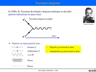
Particle Physics context for a hypothesis test A simulated SUSY event ( signal ): high pT jets of hadrons high pT muons p p missing transverse energy G. Cowan / RHUL Physics TAE 2022 Benasque (online) / Lecture day 1 23
Background events This event from Standard Model ttbar production also has high pTjets and muons, and some missing transverse energy. can easily mimic a signal event. G. Cowan / RHUL Physics TAE 2022 Benasque (online) / Lecture day 1 24
Classification of proton-proton collisions Proton-proton collisions can be considered to come in two classes: signal (the kind of event we re looking for, y = 1) background (the kind that mimics signal, y = 0) For each collision (event), we measure a collection of features: x1 = energy of muon x2 = angle between jets x3 = total jet energy x4 = missing transverse energy x5 = invariant mass of muon pair x6 = ... The real events don t come with true class labels, but computer- simulated events do. So we can have a set of simulated events that consist of a feature vector x and true class label y (0 for background, 1 for signal): (x, y)1, (x, y)2, ..., (x, y)N The simulated events are called training data . G. Cowan / RHUL Physics TAE 2022 Benasque (online) / Lecture day 1 25
Distributions of the features If we consider only two features x = (x1, x2), we can display the results in a scatter plot (red: y = 0, blue: y = 1). For real events, the dots are black (true type is not known). For each real event test the hypothesis that it is background. (Related to this: test that a sample of events is all background.) The test s critical region is defined by a decision boundary without knowing the event type, we can classify them by seeing where their measured features lie relative to the boundary. G. Cowan / RHUL Physics TAE 2022 Benasque (online) / Lecture day 1 26
Decision function, test statistic A surface in an n-dimensional space can be described by scalar function constant Different values of the constant tc result in a family of surfaces. Problem is reduced to finding the best decision function or test statistic t(x). G. Cowan / RHUL Physics TAE 2022 Benasque (online) / Lecture day 1 27
Distribution of t(x) By forming a test statistic t(x), the boundary of the critical region in the n-dimensional x-space is determined by a single single value tc. f(t|H0) f(t|H1) tc W G. Cowan / RHUL Physics TAE 2022 Benasque (online) / Lecture day 1 28
Types of decision boundaries So what is the optimal boundary for the critical region, i.e., what is the optimal test statistic t(x)? First find best t(x), later address issue of optimal size of test. Remember x-space can have many dimensions. cuts linear non-linear G. Cowan / RHUL Physics TAE 2022 Benasque (online) / Lecture day 1 29
Test statistic based on likelihood ratio How can we choose a test s critical region in an optimal way , in particular if the data space is multidimensional? For a test of H0 of size , to get the highest power with respect to the alternative H1 we need for all x in the critical region W Neyman-Pearson lemma states: likelihood ratio (LR) inside W and c outside, where c is a constant chosen to give a test of the desired size. Equivalently, optimal scalar test statistic is N.B. any monotonic function of this is leads to the same test. G. Cowan / RHUL Physics TAE 2022 Benasque (online) / Lecture day 1 30
Neyman-Pearson doesnt usually help We usually don t have explicit formulae for the pdfs f(x|s), f(x|b), so for a given xwe can t evaluate the likelihood ratio Instead we may have Monte Carlo models for signal and background processes, so we can produce simulated data: generate x ~ f(x|s) x1,..., xN generate x ~ f(x|b) x1,..., xN This gives samples of training data with events of known type. Use these to construct a statistic that is as close as possible to the optimal likelihood ratio ( Machine Learning). G. Cowan / RHUL Physics TAE 2022 Benasque (online) / Lecture day 1 31
Approximate LR from histograms Wantt(x) = f(x|s)/f(x|b) forxhere One possibility is to generate MC data and construct histograms for both signal and background. N(x|s) N(x|s) f(x|s) Use (normalized) histogram values to approximate LR: x N(x|b) N(x|b) f(x|b) Can work well for single variable. x G. Cowan / RHUL Physics TAE 2022 Benasque (online) / Lecture day 1 32
Approximate LR from 2D-histograms Suppose problem has 2 variables. Try using 2-D histograms: back- ground signal Approximate pdfs using N(x,y|s), N(x,y|b) in corresponding cells. But if we want M bins for each variable, then in n-dimensions we have Mncells; can t generate enough training data to populate. Histogram method usually not usable for n > 1 dimension. G. Cowan / RHUL Physics TAE 2022 Benasque (online) / Lecture day 1 33
Strategies for multivariate analysis Neyman-Pearson lemma gives optimal answer, but cannot be used directly, because we usually don t have f(x|s), f(x|b). Histogram method with M bins for n variables requires that we estimate Mn parameters (the values of the pdfs in each cell), so this is rarely practical. A compromise solution is to assume a certain functional form for the test statistic t(x) with fewer parameters; determine them (using MC) to give best separation between signal and background. Alternatively, try to estimate the probability densities f(x|s) and f(x|b) (with something better than histograms) and use the estimated pdfs to construct an approximate likelihood ratio. G. Cowan / RHUL Physics TAE 2022 Benasque (online) / Lecture day 1 34
Multivariate methods (Machine Learning) Many new (and some old) methods: Fisher discriminant (Deep) Neural Networks Kernel density methods Support Vector Machines Decision trees Boosting Bagging G. Cowan / RHUL Physics TAE 2022 Benasque (online) / Lecture day 1 35
Linear test statistic Suppose there are n input variables: x = (x1,..., xn). Consider a linear function: For a given choice of the coefficients w = (w1,..., wn) we will get pdfs f(y|s) and f(y|b) : G. Cowan / RHUL Physics TAE 2022 Benasque (online) / Lecture day 1 36
Linear test statistic Fisher: to get large difference between means and small widths for f(y|s) and f(y|b), maximize the difference squared of the expectation values divided by the sum of the variances: Setting J/ wi = 0 gives: , G. Cowan / RHUL Physics TAE 2022 Benasque (online) / Lecture day 1 37
The Fisher discriminant The resulting coefficients widefine a Fisher discriminant. Coefficients defined up to multiplicative constant; can also add arbitrary offset, i.e., usually define test statistic as Boundaries of the test s critical region are surfaces of constant y(x), here linear (hyperplanes): G. Cowan / RHUL Physics TAE 2022 Benasque (online) / Lecture day 1 38
Nonlinear decision boundaries From the scatter plot below it s clear that some nonlinear boundary would be better than a linear one: And to have a nonlinear boundary, the decision function t(x) must be nonlinear in x. G. Cowan / RHUL Physics TAE 2022 Benasque (online) / Lecture day 1 39
Neural Networks A simple nonlinear decision function can be constructed as where his called the activation function . For this one can use, e.g., a logistic sigmoid function, u G. Cowan / RHUL Physics TAE 2022 Benasque (online) / Lecture day 1 40
Single Layer Perceptron In this form, the decision function is called a Single Layer Perceptron the simplest example of a Neural Network. output node input layer But the surface described by t(x) = tcis the same as by So here we still have a linear decision boundary. G. Cowan / RHUL Physics TAE 2022 Benasque (online) / Lecture day 1 41
Multilayer Perceptron The Single Layer Perceptron can be generalized by defining first a set of functions i(x), with i = 1,..., m: The i(x) are then treated as if they were the input variables, in a perceptron, i.e., the decision function (output node) is G. Cowan / RHUL Physics TAE 2022 Benasque (online) / Lecture day 1 42
Multilayer Perceptron (2) output node hidden layer with m nodes 1(x),..., m(x) input layer Each line in the graph represents one of the weights wij(k), which must be adjusted using the training data. G. Cowan / RHUL Physics TAE 2022 Benasque (online) / Lecture day 1 43
Training a Neural Network To train the network (i.e., determine the best values for the weights), define a loss function, e.g., where w represents the set of all weights, the sum is over the set of training events, and yiis the (numeric) true class label of each event (0 or 1). The optimal values of the weights are found by minimizing E(w) with respect to the weights (non-trivial algorithms: backpropagation, stochastic gradient descent,...). The desired result for an event with feature vector x is: if the event is of type 0, want t(x) ~ 0, if the event is of type 1, want t(x) ~ 1. G. Cowan / RHUL Physics TAE 2022 Benasque (online) / Lecture day 1 44
Distribution of neural net output Degree of separation between classes now much better than with linear decision function: back- ground signal G. Cowan / RHUL Physics TAE 2022 Benasque (online) / Lecture day 1 45
Neural network example from LEP II Signal: e+e W+W (often 4 well separated hadron jets) Background: e+e qqgg (4 less well separated hadron jets) input variables based on jet structure, event shape, ... none by itself gives much separation. Neural network output: (Garrido, Juste and Martinez, ALEPH 96-144) G. Cowan / RHUL Physics TAE 2022 Benasque (online) / Lecture day 1 46
H.I. Kim and K.Y. Han, Water 2020, 12(3), 899 Deep Neural Networks The multilayer perceptron can be generalized to have an arbitrary number of hidden layers, with an arbitrary number of nodes in each (= network architecture ). A deep network has several (or many) hidden layers: Deep Learning is a very recent and active field of research. G. Cowan / RHUL Physics TAE 2022 Benasque (online) / Lecture day 1 47
Comments on network training The algorithms for adjusting the network parameters have become a very active field of research (and beyond the scope of this course). Recent ideas include: Deep neural nets, use of ReLU activation function Stochastic gradient descent: estimate of gradient approximated by a randomly selected subset of the data. Dropout: randomly exclude nodes during training (prevents overtraining ) G. Cowan / RHUL Physics TAE 2022 Benasque (online) / Lecture day 1 48
Overtraining Including more parameters in a classifier makes its decision boundary increasingly flexible, e.g., more nodes/layers for a neural network. A flexible classifier may conform too closely to the training points; the same boundary will not perform well on an independent test data sample ( overtraining ). independent test sample training sample G. Cowan / RHUL Physics TAE 2022 Benasque (online) / Lecture day 1 49
Monitoring overtraining If we monitor the fraction of misclassified events (or similar, e.g., error function E(w)) for test and training samples, it will usually decrease for both as the boundary is made more flexible: optimum at minimum of error rate for test sample error rate increase in error rate indicates overtraining test sample training sample flexibility (e.g., number of nodes/layers in MLP) G. Cowan / RHUL Physics TAE 2022 Benasque (online) / Lecture day 1 50


")


")
")


")


")


")


")


, 899")