Understanding Paired Data Analysis in Research Studies
This content discusses the significance of paired data, its role in reducing variability, and examples of experimental designs used in research studies. Explore comparisons between Meijer and Family Fare prices, and testing The Freshmen 15 theory. Discover how different music types affect studying and experimental designs for studying with music.

Uploaded on Oct 04, 2024 | 0 Views
Download Presentation

Please find below an Image/Link to download the presentation.
The content on the website is provided AS IS for your information and personal use only. It may not be sold, licensed, or shared on other websites without obtaining consent from the author. Download presentation by click this link. If you encounter any issues during the download, it is possible that the publisher has removed the file from their server.
E N D
Presentation Transcript
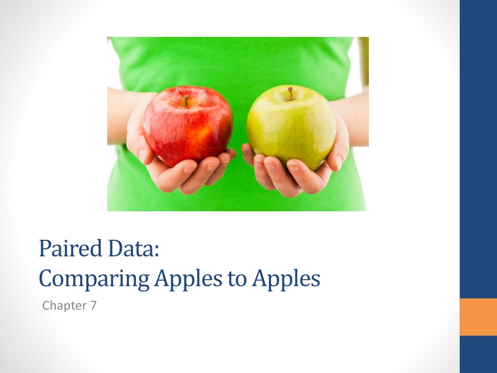
Paired Data: Comparing Apples to Apples Chapter 7
What would you do? How would you go about collecting your data for each of the following. You want to compare grocery prices between Meijer and Family Fare. Are prices different, on average? You want to test The Freshmen 15 theory. Do college students gain, on average, 15 pounds during their first year?
Introduction The paired datasets in this chapter have one pair of quantitative response values for each observational unit. This allows for a built-in comparison. Studies with paired data remove individual variability by looking at the difference score for each individual. Reducing variability in data improves inferences: Narrower confidence intervals Smaller p-values when the null hypothesis is false
Can You Study With Music Blaring? Example 7.1
Studying with Music Many students study while listening to music. Does it hurt their ability to focus? In Checking It Out: Does music interfere with studying? Stanford Prof Clifford Nass claims the human brain listens to song lyrics with the same part that does word processing Instrumental music is, for the most part, processed on the other side of the brain and Nass claims that reading and listening to instrumental music has virtually no interference.
Studying with Music Consider the experimental designs: Experiment 1 Random assignment to 2 groups 27 students were randomly assigned to 1 of 2 groups: One group listens to music with lyrics One group listens to music without lyrics Students play a memorization game while listening to the particular music that they were assigned.
Studying with Music Experiment 2 Paired design using repeated measures All students play the memorization game twice: Once while listening to music with lyrics Once while listening to music without lyrics. Experiment 3 Paired design using matching Sometimes repeating something is impossible (like testing a surgical procedure) but we can still pair. Test each student on memorization. Match students up with similar scores and randomly: Have one play the game while listening to music with lyrics and the other while listening to music without lyrics.
Studying with Music Suppose we ended up with the results shown below. If we analyzed this like we did in chapter 6, we should see that: One distribution is a bit higher than the other, but not much higher There is quite a bit of overlap in the data The resulting p-value will not be very small Without Lyrics With Lyrics
Studying with Music Now, what if I told you this test was done twice on the same set of 27 students? Everyone could remember exactly 2 more words when they listened to a song without lyrics. We don t see the connection in the points below. Without Lyrics With Lyrics
Studying with Music The results from the applet below show the connection between the pairs of scores. From the lines we can see that all scores in the top graph are two more than those in the bottom graph and that these pairs are from the same person.
Studying with Music We really need to focus on the difference in scores and these differences are all the same. Do these differences look significantly larger than 0?
Studying with Music Variability in people s memorization abilities may make it difficult to see differences between the songs in the first experiment. The paired design focuses on the difference in the number of words memorized, instead of the number of words memorized. By looking at this difference, the variability in general memorization ability is taken away.
Pairing and Random Assignment Pairing often makes it easier to detect statistical significance Can we still make cause-and-effect conclusions in paired design? Can we still have random assignment?
Pairing and Random Assignment In our memorizing with or without lyrics example: If we see significant improvement in performance, is it attributable to the type of song? What about experience? Could that have made the difference? What is a better design? Randomly assign each person to which song they hear first: with lyrics first, or without. This cancels out an experience effect
Paring and Observational Studies We can use pairing in observational studies. If you are interested in which test was more difficult in a course, the first or the second, compare the average difference in scores for each individual. Use a Pretest and a Postest.
Learning Objects for Sections 7.1 Understand the difference between independent samples and paired samples in terms of the study design Understand how variability can be lower in a paired design and how this can influence the strength of evidence.
Section 7.2: Simulation-Based Approach for Analyzing Paired Data Example 7.2: Rounding First Base
Rounding First Base Imagine you ve hit a line drive and are trying to reach second base. Does the path that you take to round first base make much of a difference? Narrow angle Wide angle Narrow Wide
Rounding First Base Woodward (1970) investigated these base running strategies. He timed 22 different runners from a spot 35 feet past home to a spot 15 feet before second. Each runner used each strategy (paired design), with a rest between. He used random assignment to decide which path each runner should do first. This paired design controls for the runner-to-runner variability.
First Base What are the observational units in this study? The runners (22 total) What variables are recorded? What are their types and roles? Explanatory variable: base running method: wide or narrow angle (categorical) Response variable: time for middle of the route from home plate to second base (quantitative) Is this an observational study or an experiment? Randomized experiment since the explanatory variable was randomly applied to determined which method each runner used first.
The Statistics There is a lot of overlap in the distributions and a fair bit of variability Mean 5.534 SD 0.260 Narrow Wide 5.459 0.273 Difficult to detect a difference between the methods when there s a lot of variation
Rounding First Base However, these data are clearly paired. The paired response variable is time difference in running between the two methods and this is how the data need to be explored and analyzed.
The Differences in Times Mean difference is ?d = 0.075 seconds Standard deviation is SDd = 0.0883 sec Standard deviation (0.0883) is smaller than the original standard deviations of the running times (0.260 and 0.273).
Rounding First Base Below are the original dotplots with each observation paired between the base running strategies. What do you notice?
Rounding First Base Is the average difference of ?d = 0.075 seconds significantly different from 0? The parameter of interest, d, is the long run mean difference in running times for runners using the narrow angled path instead of the wide angled path. (narrow wide)
Rounding First Base The hypotheses: H0: d = 0 The long run mean difference in running times is 0. Ha: d 0 The long run mean difference in running times is not 0. The statistic ?d = 0.075 is above zero, but we need to ask the same question we ve asked before: How likely is it to see such a large average difference in running times by chance alone, even if the base running strategy has no genuine effect on the times?
Rounding First Base How can we use simulation-based methods find an approximate p-value? The null basically says the running path doesn t matter. So we can use our same data set and, for each runner, randomly decide which time goes with the narrow path and which time goes with the wide path and then compute the difference. (Notice we don t break our pairs.) After we do this for each of runner, we then compute a mean difference. We will then repeat this process many times to develop a null distribution.
Random Swapping Subject narrow angle wide angle diff 1 2 3 4 5 6 7 8 9 10 5.80 5.70 -0.10 11 5.60 5.50 5.50 5.55 -0.05 0.05 5.50 5.35 5.55 5.60 -0.05 5.40 5.35 0.05 5.70 5.75 -0.05 5.50 5.40 0.10 5.85 5.70 0.15 5.15 5.00 0.15 5.20 5.10 0.10 0.10 -0.10 0.15 -0.15 0.10 Subject narrow angle wide angle diff 12 5.50 5.45 0.05 13 14 15 16 17 5.55 5.35 -0.20 18 19 5.45 5.25 -0.20 20 21 22 5.35 5.45 -0.10 5.00 4.95 0.05 5.50 5.40 0.10 5.55 5.50 0.05 5.50 5.55 -0.05 5.60 5.40 0.20 5.65 5.55 0.10 6.30 6.25 0.05 0.20 0.20 ?d = 0.011
More Simulations -0.002 -0.002 0.002 -0.007 0.030 -0.011 0.016 0.002 -0.007 -0.016 0.020 -0.002 -0.067 -0.007 0.007 With 26 repetitions of creating simulated mean differences, we did not get any that were as extreme as 0.075. 0.467 -0.034 0.002 -0.016 -0.030 0.020 0.066 -0.025 -0.002 -0.002 -0.075 0.075 Simulated Mean Differences
First Base Here is a null distribution of 1000 simulated mean differences Where s the center? Where s our observed statistic of 0.075?
First Base Only 1 of the 1000 repetitions of random swappings gave a ?? value at least as extreme as 0.075
First Base We can also standardize 0.075 by dividing by the applet s estimate of the SD 0.024 to see we are 0.075 3.125 standard deviations above zero. 0.024=
Rounding First Base With a p-value of 0.001, we have very strong evidence against the null hypothesis and can conclude that the running path does matter with the wide-angle path being faster, on average. We can draw a cause-and-effect conclusion since the researcher used random assignment of the two base running methods for each runner. There was not a lot of information about how these 22 runners were selected to decide if we can generalize to a larger population.
3S Strategy Statistic: Compute the statistic in the sample. In this case, the statistic we looked at was the observed mean difference in running times. Simulate: Identify a chance model that reflects the null hypothesis. We tossed a coin for each runner, and if it landed heads we swapped the two running times for that runner. If the coin landed tails, we did not swap the times. We then computed the mean difference for the 22 runners and repeated this process many times. Strength of evidence: We found that only 1 out of 1000 of our simulated mean differences was at least as extreme as the observed difference of 0.075 seconds.
First Base Approximate a 95% confidence interval for ?d: 0.075 2(0.024) seconds (0.027, 0.124) seconds What does this mean? We are 95% confident that, on average, the narrow angle route takes 0.027 to 0.124 seconds longer than the wide angle route
First Base Alternative Analysis What do you think would happen if we wrongly analyzed the data using a 2 independent samples procedure? (i.e. The researcher selected 22 runners to use the wide method and an independent sample of 22 other runners to use the narrow method, obtaining the same 44 times as in the actual study.
First Base Using the Multiple Means applet (which does an independent test) we get a p-value of 0.3470. Does it make sense that this p-value is larger than the one we obtained earlier?
Applet Let s look at the baseball example in the applet. The data is already loaded into the Matched Pairs applet. Run the test and get a p-value and standardized statistic. Find an approximate 95% confidence interval (2SD)
Learning Objects for Sections 7.2 Describe the simulation process for a matched pairs test. Complete a simulation-based test of significance of a paired design by writing out the hypothesis, determining the observed statistic, computing the p-value, and writing out an appropriate conclusion. Compute a 2SD confidence interval for the mean difference and a standardized statistic and relate these to the results of a test of significance.
Exercise and Heart Rate Which will result in a higher heart rate, doing jumping jacks and bicycle kicks? Exploration 7.2 page 395.
Theory-based Approach for Analyzing Data from Paired Samples Section 7.3
How Many M&Ms Would You Like? Does your bowl size affect how much you eat? Brian Wansink studied this question with college students over several days. At one session, the 17 participants were assigned to receive either a small bowl or a large bowl and were allowed to take as many M&Ms as they would like. At the following session, the bowl sizes were switched for each participant.
How Many M&Ms Would You Like? What are the observational units? What is the explanatory variable? What is the response variable? Is this an experiment or an observational study? Will the resulting data be paired?
How Many M&Ms Would You Like? The hypotheses: H0: d = 0 The long-run mean difference in number of M&Ms taken (small large) is 0. Ha: d< 0 The long-run mean difference in number of M&Ms taken (small large) is less than 0.
How Many M&Ms Would You Like? Here are the results of a simulation-based test. The p-value is quite large at 0.1220.
How Many M&Ms Would You Like? Our null distribution was centered at zero and fairly bell-shaped. This can all be predicted (along with the variability) using theory-based methods. Theory-based methods should be valid if the population distribution of differences is symmetric (we can guess at this by looking at the sample distribution of differences) or our sample size is at least 20. Our sample size was only 17, but this distribution of differences is fairly symmetric, so we will proceed with a theory-based test.
Theory-based test We can do theory-based methods with the applet we used last time or the theory-based applet. With the applet we used last time, we need to calculate the t-statistic: ?? ? = ?? ? With the theory-based applet, we just need to enter the summary statistics and use a test for a one mean. This kind of test is called a paired t-test.