Comparing Average in Different Groups: Paired vs. Independent Samples
In statistical analysis, comparing averages in different groups is essential for various research scenarios. This involves distinguishing between paired observations and independent samples, leading to different t-tests for analysis. Understanding these concepts is crucial for making accurate comparisons based on continuous variables across groups. The process involves considering factors like treatment effects, gender disparities, and experimental conditions to draw meaningful conclusions from the data.

Download Presentation

Please find below an Image/Link to download the presentation.
The content on the website is provided AS IS for your information and personal use only. It may not be sold, licensed, or shared on other websites without obtaining consent from the author. Download presentation by click this link. If you encounter any issues during the download, it is possible that the publisher has removed the file from their server.
E N D
Presentation Transcript
Part 2 - Compare average in different groups
Comparing average Often we want to compare the average of a continuous variable in different groups. Examples: Continuous variable Categorical variable Height Before and after a treatment Weight Treatment and placebo Bloodbpressure Men and women Triglycerides in blood Two different treatments CD4 counts Sick and healthy Cholesterol Normal and overweight .. .. 2
Paired or independent sample When comparing the average in different groups, we must distinguish between two different layouts: - Paired observations; The same individual is measured twice. Example: before and after treatment. - Independent samples; two independent groups of individuals have been measured. Example: treatment and placebo. 3
Paired or independent sample When comparing the average in different groups, we must distinguish between two different layouts: - Paired observations; The same individual is measured twice. - Independent samples; two independent groups of individuals have been measured. This gives two different t-tests: Paired sample t-test Independent sample t-test 4
Example Paired Observations Independent Samples Before and after treatment Men and women Two different treatments on the same subject Treatment and placebo in two independent groups Treatment and placebo with identical twins Case and control 5
Paired or independent sample in SPSS We need to set up the data differently for the paired and the independent setup. Paired Independent 6
T-test & normality If the variables are approximately normal T-test 7
T-test & normality If the variables are approximately normal T-test If the variables are far from normality Non-parametric test Transformation of data (ex: log-scale) 8
T-test & normality If the variables are approximately normal T-test If the variables are far from normal Non-parametric test Transformation of data (ex: log-scale) Check for normality with visual plots: 1. Histogram (one peak, simmetry) 2. Boxplot (simmetry) 3. QQ-plot (in line, withouth heavy tails ) 9
T-test for one sample A one-sample T-test of the average of a variable equals to a certain value Go to Analyze > Compare Means > One Sample T-test 10
T-test for one sample A one-sample T-test of the average of a variable equals to a certain value Go to Analyze > Compare Means > One Sample T-test Enter the value you want to test in Test Value . 11
T-test for one sample A one-sample T-test of the average of a variable equals to a certain value Go to Analyze > Compare Means > One Sample T-test Enter the value you want to test in Test Value . Click Options , and set 95% CI. 12
T-test for one sample A one-sample T-test of the average of a variable equals to a certain value Go to Analyze > Compare Means > One Sample T-test Enter the value you want to test in Test Value . Click Options , and set 95% CI. Click Continue and OK in the previous box. 13
Paired-Samples T-test We want to test if there are significant differences in blood pressure at two measurements. To use the t-test, we need to check the normality, but for a paired sample we have to check that the difference between measurements is normally distributed. First, create a variable with the difference: Transform => Compute variable 14
Enter new variable name: DiffBP. NB! The name can not contain spaces. 15
Enter new variable name: DiffBP. NB! The name can not contain spaces. Write the desired transformation in Numeric Expression: BPafter BPbas 16
Enter new variable name: DiffBP. NB! The name can not contain spaces. Alternatively... Here you can also select variables in the table and double-click / drag. 17
Enter new variable name: DiffBP. NB! The name can not contain spaces. Write the desired transformation in Numeric Expression: NB! if any of the cells for one of the variables are missing, the difference will also be missing BPafter BPbas Click OK 18
Then we can create histogram, boxplot and QQ-plot for the difference DiffBP (as in Part 1). Normality seems to be fulfilled: T-test works fine! On the line Simmetric One peak 19
Paired-Samples T Test We want to test if there is a significant difference in blood pressure before and after a treatment. Go to Analyze => Compare means => Paired-Samples T-test 20
Paired-Samples T Test We want to test if there is a significant difference in blood pressure before and after a treatment. Go to Analyze => Compare means => Paired-Samples T-test Move BPbas to Variable1 and BPafter to Variable2. 21
Paired-Samples T Test We want to test if there is a significant difference in blood pressure before and after a treatment. Go to Analyze => Compare means => Paired-Samples T-test Move BPbas to Variable1 and BPafter to Variable2. Click OK . 22
Paired sample T Test output First we have average and standard deviation (SD) for the two samples 24
Paired sample T Test output Then we have the test of the difference: mean differance between before and after 25
Paired sample T Test output The P-value of the test is bigger than 0.05, so it is not significant. This imply that the mean difference is equal to 0. 26
Paired sample T Test output Note: Confidence Interval for the means difference. NB - SPSS tests the difference Variable1 - Variable2, so Beforeminus After, then an increase of the average will give a negative difference. If you want to invert, you have to select After as Variable1 and Before as Variable2. 27
Exercise 2a The Caerphilly study measured total cholesterol in two different visits ( totchol and totchol2 ). Check if there is a significant difference in total cholesterol between first and second visits. Hint: Check for normality Paired samples T test 28
Exercise 2a - Solution Step 1: Normality plot of difference => Assuming normality is fine. 29
Steg 2: Paired samples T test The P-value is over 0.05: the difference of the total cholesterol between visit 1 and visit 2 is non-significant. 31
Independent Samples T test We want to test if the average in two different groups is different: eg. blood pressure measured in smokers and non-smokers. If the variable in both groups can be assumed to be normal, you can use: Independent Samples T test. 32
How to check normality? Remember! When the variable is measured in independent groups, the data file must be organized in a variable column and a group-indicator column. Data file needs to be re-structured if necessary! 33
How to check normality? Remember! When the variable is measured in independent groups, the data file must be organized in a variable column and a group-indicator column. Analyze => Descriptive Statistics => Explore move group-indicator to Factor List. 34
How to check normality? Remember! When the variable is measured in independent groups, the data file must be organized in a variable column and a group-indicator column. Analyze => Descriptive Statistics => Explore move group-indicator to Factor List. Click Plots and removes Stem-and-leaf . Select Histogram and Normality plots with test , as in Part 1. 35
How to check normality? Remember! When the variable is measured in independent groups, the data file must be organized in a variable column and a group-indicator column. Analyze => Descriptive Statistics => Explore move group-indicator to Factor List. Click Plots and removes Stem-and-leaf . Select Histogram and Normality plots with test , as in Part 1. 36
Normality plot for the two groups (Smoker / Non-smoker) separately: Non-smoker Smoker 37
Normality plot for the two groups (Smoker / Non-smoker) separately: Non-smoker Smoker It seems possible to assume normality in both groups. 38
To test the difference of the two averages: Go to Analyze => Compare Means => Independent Samples T test 39
To test the difference of the two averages: Go to Analyze => Compare Means => Independent Samples T test Move the continuous variable (BPbas) to Test Variable(s) 40
To test the difference of the two averages: Go to Analyze => Compare Means => Independent Samples T test Move the continuous variable (BPbas) to Test Variable(s) and group-indicator (Smoker) to Grouping Variable , click Define Groups 41
To test the difference of the two averages: Go to Analyze => Compare Means => Independent Samples T test Move the continuous variable (BPbas) to Test Variable(s) and group-indicator (Smoker) to Grouping Variable , click Define Groups Group-indicator is defined Smoker=1 , non-smoker=0 (check in Variable view): Write 0 in Group 1 42
To test the difference of the two averages: Go to Analyze => Compare Means => Independent Samples T test Move the continuous variable (BPbas) to Test Variable(s) and group-indicator (Smoker) to Grouping Variable , click Define Groups Group-indicator is defined Smoker=1 , non-smoker=0 (check in Variable view): write 0 in Group 1 write 1 in Group 2 43
To test the difference of the two averages: Go to Analyze => Compare Means => Independent Samples T test Move the continuous variable (BPbas) to Test Variable(s) and group-indicator (Smoker) to Grouping Variable , click Define Groups Group-indicator is defined Smoker=1 , non-smoker=0 (check in Variable view): write 0 in Group 1 write 1 in Group 2 Continue and OK 44
Independent Samples T test is calculated for two cases: equal or different variance in the two groups. Levene s test check the null hypotesis of equal variance. 45
Independent Samples T test is calculated for two cases: equal or different variance in the two groups. Levene s test check the null hypotesis of equal variance. If the p-value > 0.05 the variance is equal, 46
Independent Samples T test is calculated for two cases: equal or different variance in the two groups. Levene s test check the null hypotesis of equal variance. If the p-value > 0.05 the variance is equal, then read the first line (of the Independent Samples T test) 47
Independent Samples T test is calculated for two cases: equal or different variance in the two groups. Levene s test check the null hypotesis of equal variance. If the p-value > 0.05 the variance is equal, then read the first line If the p-value < 0.05 the variance is different, 48
Independent Samples T test is calculated for two cases: equal or different variance in the two groups. Levene s test check the null hypotesis of equal variance. If the p-value > 0.05 the variance is equal, then read the first line If the p-value < 0.05 the variance is different, then read the second line (of the Independent Samples T test) 49
For systolic blood pressure in smokers and non-smokers, Levene's test is not significant (p = 0.7). So, we assume equal variance in the two groups 50