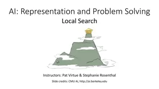
Understanding Local Search Algorithms for Optimization
Local search methods like hill climbing and simulated annealing focus on evaluating and modifying current states to find optimal solutions efficiently, making them suitable for complex state spaces. Hill climbing involves iteratively moving towards higher value states, while simulated annealing uses probabilistic transitions, avoiding local optima. Despite their advantages, these methods have limitations like getting stuck at local maxima or facing ridge and plateau problems. Various variations like stochastic hill climbing and random restarts help overcome these challenges and enhance search efficiency.

Download Presentation

Please find below an Image/Link to download the presentation.
The content on the website is provided AS IS for your information and personal use only. It may not be sold, licensed, or shared on other websites without obtaining consent from the author. Download presentation by click this link. If you encounter any issues during the download, it is possible that the publisher has removed the file from their server.
E N D
Presentation Transcript
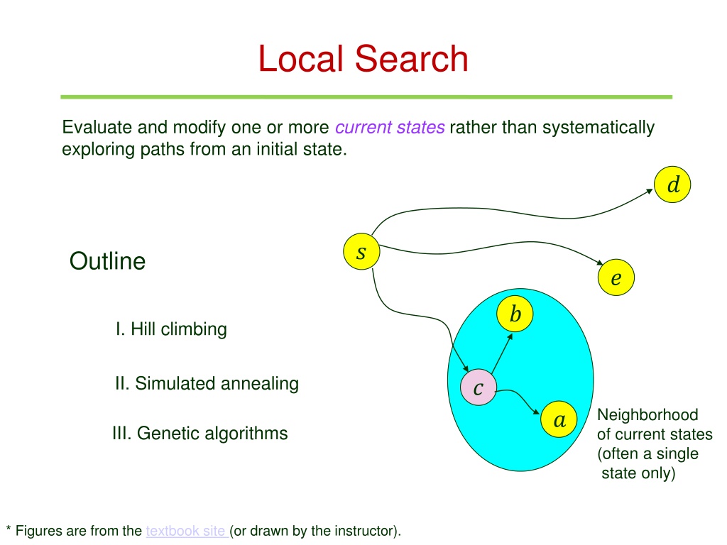
Local Search Evaluate and modify one or more current states rather than systematically exploring paths from an initial state. ? ? Outline ? ? I. Hill climbing II. Simulated annealing ? Neighborhood of current states (often a single state only) ? III. Genetic algorithms * Figures are from the textbook site (or drawn by the instructor).
Advantages of Local Search Use of very little memory. Finding good solutions in state spaces intractable for a systematic search. Useful in pure optimization (e.g., gradient-based descent methods) Maximize ?(?,?) Steepest ascent (along ? = ? ?,? = ?4 ?? ??,?? ??) ? ?,? = ?3 ?1> ?2> ?3 > ?4 ? ?,? = ?2 (level curve) ? ?,? = ?1
State Space Landscape Weighted A* search (? = 2 on the same grid)
I. Hill Climbing // random choice // to break a tile 8-queens problem s = # pairs of queens attacking each other, directly or indirectly, in the state ?. Successor is a state generated from relocating a queen in the same column. s = 12 for the best successor. 8-way tie!. Hill climbing randomly picks one. = 17
Efficiency? 5 moves = 1 Hill climbing can make rapid progress toward a solution.
Drawback of Hill Climbing (1) Hill climbing terminates when a peak is reached with no neighbor having a higher value. Local maximum Not the global maximum. Hill climbing in the vicinity of a local maximum will be drawn toward it and then get stuck there. Every move of one queen introduces more conflicts.
Drawback of Hill Climbing (2) Ridge: A sequence of local maxima difficult to navigate. At each local maximum, all available actions are downhill. Plateaus: No uphill actions exist.
Variations of Hill Climbing Stochastic hill climbing Random selection among the uphill moves. Probability of selection varying with steepness.. First-choice hill climbing Random generation of successors until a better (than the current) one is found. Useful when many successors exist and/or the objective function is costly to evaluate. Random restart hill climbing Restart search from random initial state.
II. Simulated Annealing Annealing: Heat a metal to a high temperature and then gradually cool it, allowing the material to reach a low-energy crystalline state so it is hardened. Start by shaking hard (i.e., at high temperature). Gradually reduce the intensity of shaking (i.e., lower the temperature). * from http://www.cs.us.es/~fsancho/?e=206
Simulated Annealing Algorithm Minimization Temperature lim ? ? = 0 // solution Badness Is ?. // the next state is better; choose it. . ? ?/? // ? 0 Accept the next state if it is an improvement ( ? > 0). Otherwise, accept it with a probability that decreases exponentially as the badness ? of the move increases, and Bad moves are more tolerated at the start when ? is high, and become less likely as ? decreases. as the temperature goes down. Escape local minima by allowing bad moves.
More About SA ? 0 slowly enough A property of Boltzmann distribution ? ?/? guarantees the global minimum with probability 1. Commonly used ? ?? with constant ?< 1 and close to 1 at each step. Applied to many problems: VLSL layout factory scheduling aircraft trajectory planning NP-hard optimization (i.e., the traveling salesman problem) large-scale stochastic optimization tasks
Local Beam Search Keep track of ? states rather than one. 1. Start with ? randomly generated states. ? 2. Generate all their successors. 3. Stop if any successor is a goal. 4. Otherwise, keep the ? best successors and go back to step 2. May suffer from a lack of diversity among the ? states. Solution: stochastic beam search which chooses successors with probabilities proportional to their values.
III. Evolutionary Algorithms Also called genetic algorithms. Inspired by natural selection in biology. 1. Start with a population of ? randomly generated states (individuals). 2. Select the most fit individuals to become parents of the next generation 3. Combine every ? parents to form an offspring (typically ? = 2). Crossover: Split each of the parent strings and recombine the parts to form two children. Mutation: Randomly change the bits of an offspring. Culling: All individuals below a threshold are discarded from the population. 4. Go back to step 2 and repeat until sufficiently fit states are discovered (in which case the best one is chosen as a solution).
Genetic Algorithm on 8-Queen Score = # non-attacking pairs of queens Row number of the the queen in column 1 11 14% = 24 + 23 + 20 + 11 Move the queen in column 8 to a random square (7).
Crossover 1 2 3 4 5 6 7 8 8 7 6 5 4 3 2 1
Applications of GA Complex structured problems Circuit layout, job-shop scheduling Evolving the architecture of deep neural networks Finding bugs of hardware Molecular structure optimization Image processing. Learning robots, etc.


")
")


")