Introduction to A* Algorithm and Local Search Techniques in Python
Explore the implementation of the A* algorithm in Python for solving pathfinding problems, including the use of a priority queue for the Open list. Additionally, delve into local search algorithms such as Hill Climbing and Simulated Annealing for optimization problems. Design custom data sets, run algorithms on them, and present the results alongside source code and visual representations.

Download Presentation

Please find below an Image/Link to download the presentation.
The content on the website is provided AS IS for your information and personal use only. It may not be sold, licensed, or shared on other websites without obtaining consent from the author. Download presentation by click this link. If you encounter any issues during the download, it is possible that the publisher has removed the file from their server.
E N D
Presentation Transcript
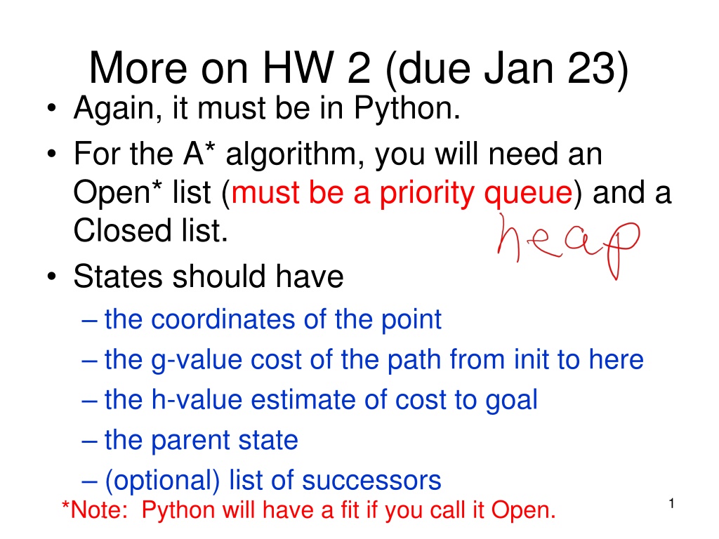
More on HW 2 (due Jan 23) Again, it must be in Python. For the A* algorithm, you will need an Open* list (must be a priority queue) and a Closed list. States should have the coordinates of the point the g-value cost of the path from init to here the h-value estimate of cost to goal the parent state (optional) list of successors *Note: Python will have a fit if you call it Open. 1
Input format Example 0 0 9 6 2 0 0 4 0 4 4 0 4 7 4 9 6 4 10 2 8 Start Point Goal Point How many Rectangles. Rectangle coordinates are given clockwise. 2
More Difficult Example Has 4 known solutions with approximately the same cost. You will just find 1 least cost solution and print the whole path with states and cumulative costs. 3
In Addition You must design your own custom data set and run your program on it, too. You will turn in a picture of your data set, similar to the pictures we give you of ours. Turn in commented source code, input and output from all 3 data sets, and your picture. 4
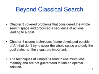
Beyond Classical Search Chapter 3 covered problems that considered the whole search space and produced a sequence of actions leading to a goal. Chapter 4 covers techniques (some developed outside of AI) that don t try to cover the whole space and only the goal state, not the steps, are important. The techniques of Chapter 4 tend to use much less memory and are not guaranteed to find an optimal solution. 5
More Search Methods Local Search Hill Climbing Simulated Annealing Beam Search Genetic Search Local Search in Continuous Spaces Searching with Nondeterministic Actions Online Search (agent is executing actions) 6
Local Search Algorithms and Optimization Problems Complete state formulation For example, for the 8 queens problem, all 8 queens are on the board and need to be moved around to get to a goal state Equivalent to optimization problems often found in science and engineering Start somewhere and try to get to the solution from there Local search around the current state to decide where to go next 7
Pose Estimation Example Given a geometric model of a 3D object and a 2D image of the object. Determine the position and orientation of the object wrt the camera that snapped the image. image 3D object State (x, y, z, x, y, z) 8
Gradient What is the gradient of a function? In 1D. Function f(x). Gradient f (x), the derivative. In 2D. Function f(x,y). Gradient ( x, y) e.g. f(x) = x2. f (x) = ? 9
Hill Climbing Gradient ascent solution Note: solutions shown here as max not min. Often used for numerical optimization problems. How does it work? In continuous space, the gradient tells you the direction in which to move uphill. 10
Numeric Example -1 0 1 Normal distribution with 0 mean and 1 SD f(x) = c e ^ (-1/2)x2 f (x) = -x c e ^ (-1/2)x2 f (1) comes out negative, ie. move backward f (-1) comes out positive, ie. move forward. 11
AI Hill Climbing Steepest-Ascent Hill Climbing current start node loop do neighbor a highest-valued successor of current if neighbor.Value <= current.Value then return current.State current neighbor end loop At each step, the current node is replaced by the best (highest-valued) neighbor. This is sometimes called greedy local search. 12
Hill Climbing Search current 6 4 10 3 2 8 What if current had a value of 12? 13
Hill Climbing Problems Local maxima Plateaus Diagonal ridges What is it sensitive to? Does it have any advantages? 14
Solving the Problems Allow backtracking (What happens to complexity?) Stochastic hill climbing: choose at random from uphill moves, using steepness for a probability Random restarts: If at first you don t succeed, try, try again. Several moves in each of several directions, then test Jump to a different part of the search space 15
Simulated Annealing Variant of hill climbing (so up is good) Tries to explore enough of the search space early on, so that the final solution is less sensitive to the start state May make some downhill moves before finding a good way to move uphill. 16
Simulated Annealing Comes from the physical process of annealing in which substances are raised to high energy levels (melted) and then cooled to solid state. heat cool The probability of moving to a higher energy state, instead of lower is p = e^(- E/kT) where E is the positive change in energy level, T is the temperature, and k is Bolzmann s constant. 17
Simulated Annealing At the beginning, the temperature is high. As the temperature becomes lower kT becomes lower E/kT gets bigger (- E/kT) gets smaller e^(- E/kT) gets smaller As the process continues, the probability of a downhill move gets smaller and smaller. 18
For Simulated Annealing E represents the change in the value of the objective function. Since the physical relationships no longer apply, drop k. So p = e^(- E/T) We need an annealing schedule, which is a sequence of values of T: T0, T1, T2, ... 19
Simulated Annealing Algorithm current start node; for each T on the schedule /* need a schedule */ next randomly selected successor of current evaluate next; if it s a goal, return it E next.Value current.Value if E > 0 then current next else current next with probability e^( E/T) /* already negated */ /* better than current */ How would you do this probabilistic selection? 20
Probabilistic Selection Select next with probability p p 0 1 random number Generate a random number If it s <= p, select next 21
Simulated Annealing Properties At a fixed temperature T, state occupation probability reaches the Boltzman distribution p(x) = e^(E(x)/kT) If T is decreased slowly enough (very slowly), the procedure will reach the best state. Slowly enough has proven too slow for some researchers who have developed alternate schedules. 22
Simulated Annealing Schedules Acceptance criterion and cooling schedule 23
Simulated Annealing Applications Basic Problems Traveling salesman Graph partitioning Matching problems Graph coloring Scheduling Engineering VLSI design Placement Routing Array logic minimization Layout Facilities layout Image processing Code design in information theory 24
Local Beam Search Keeps more previous states in memory Simulated annealing just kept one previous state in memory. This search keeps k states in memory. - randomly generate k initial states - if any state is a goal, terminate - else, generate all successors and select best k - repeat 25
Coming next: Genetic Algorithms, which are motivated by human genetics. How do you search a very large search space in a fitness oriented way? 27
")