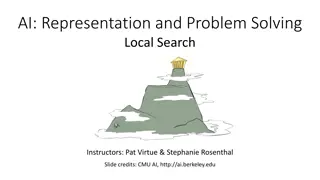
Techniques in Beyond Classical Search and Local Search Algorithms
The chapter discusses search problems that consider the entire search space and lead to a sequence of actions towards a goal. Chapter 4 explores techniques, including Hill Climbing, Simulated Annealing, and Genetic Search, focusing solely on the goal state rather than the entire space. These methods require less memory but do not guarantee optimal solutions. It delves into Local Search Algorithms and Optimization Problems, highlighting complete state formulation and the application of local search to decision-making. The concept of Pose Estimation Example and Hill Climbing's use in numerical optimization problems are also covered.

Download Presentation

Please find below an Image/Link to download the presentation.
The content on the website is provided AS IS for your information and personal use only. It may not be sold, licensed, or shared on other websites without obtaining consent from the author. Download presentation by click this link. If you encounter any issues during the download, it is possible that the publisher has removed the file from their server.
E N D
Presentation Transcript
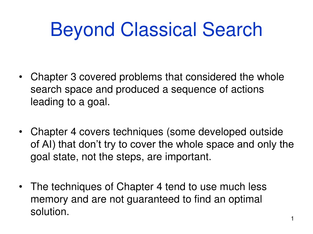
Beyond Classical Search Chapter 3 covered problems that considered the whole search space and produced a sequence of actions leading to a goal. Chapter 4 covers techniques (some developed outside of AI) that don t try to cover the whole space and only the goal state, not the steps, are important. The techniques of Chapter 4 tend to use much less memory and are not guaranteed to find an optimal solution. 1
More Search Methods Local Search Hill Climbing Simulated Annealing Beam Search Genetic Search Local Search in Continuous Spaces Searching with Nondeterministic Actions Online Search (agent is executing actions) 2
Local Search Algorithms and Optimization Problems Complete state formulation For example, for the 8 queens problem, all 8 queens are on the board and need to be moved around to get to a goal state Equivalent to optimization problems often found in science and engineering Start somewhere and try to get to the solution from there Local search around the current state to decide where to go next 3
Pose Estimation Example Given a geometric model of a 3D object and a 2D image of the object. Determine the position and orientation of the object wrt the camera that snapped the image. image 3D object State (x, y, z, x, y, z) 4
Hill Climbing Gradient ascent solution Note: solutions shown here as max not min. Often used for numerical optimization problems. How does it work? In continuous space, the gradient tells you the direction in which to move uphill. 5
AI Hill Climbing Steepest-Ascent Hill Climbing current start node loop do neighbor a highest-valued successor of current if neighbor.Value <= current.Value then return current.State current neighbor end loop At each step, the current node is replaced by the best (highest-valued) neighbor. This is sometimes called greedy local search. 6
Hill Climbing Search current 6 4 10 3 2 8 What if current had a value of 12? 7
Hill Climbing Problems Local maxima Plateaus Diagonal ridges What is it sensitive to? Does it have any advantages? 8
Solving the Problems Allow backtracking (What happens to complexity?) Stochastic hill climbing: choose at random from uphill moves, using steepness for a probability Random restarts: If at first you don t succeed, try, try again. Several moves in each of several directions, then test Jump to a different part of the search space 9
Simulated Annealing Variant of hill climbing (so up is good) Tries to explore enough of the search space early on, so that the final solution is less sensitive to the start state May make some downhill moves before finding a good way to move uphill. 10
Simulated Annealing Comes from the physical process of annealing in which substances are raised to high energy levels (melted) and then cooled to solid state. heat cool The probability of moving to a higher energy state, instead of lower is p = e^(- E/kT) where E is the positive change in energy level, T is the temperature, and k is Bolzmann s constant. 11
Simulated Annealing At the beginning, the temperature is high. As the temperature becomes lower kT becomes lower E/kT gets bigger (- E/kT) gets smaller e^(- E/kT) gets smaller As the process continues, the probability of a downhill move gets smaller and smaller. 12
For Simulated Annealing E represents the change in the value of the objective function. Since the physical relationships no longer apply, drop k. So p = e^(- E/T) We need an annealing schedule, which is a sequence of values of T: T0, T1, T2, ... 13
Simulated Annealing Algorithm current start node; for each T on the schedule /* need a schedule */ next randomly selected successor of current evaluate next; it it s a goal, return it E next.Value current.Value if E > 0 then current next else current next with probability e^( E/T) /* already negated */ /* better than current */ How would you do this probabilistic selection? 14
Probabilistic Selection Select next with probability p p 0 1 random number Generate a random number If it s <= p, select next 15
Simulated Annealing Properties At a fixed temperature T, state occupation probability reaches the Boltzman distribution p(x) = e^(E(x)/kT) If T is decreased slowly enough (very slowly), the procedure will reach the best state. Slowly enough has proven too slow for some researchers who have developed alternate schedules. 16
Simulated Annealing Schedules Acceptance criterion and cooling schedule 17
Simulated Annealing Applications Basic Problems Traveling salesman Graph partitioning Matching problems Graph coloring Scheduling Engineering VLSI design Placement Routing Array logic minimization Layout Facilities layout Image processing Code design in information theory 18
Local Beam Search Keeps more previous states in memory Simulated annealing just kept one previous state in memory. This search keeps k states in memory. - randomly generate k initial states - if any state is a goal, terminate - else, generate all successors and select best k - repeat 19
Genetic Algorithms Start with random population of states Representation serialized (ie. strings of characters or bits) States are ranked with fitness function Produce new generation Select random pair(s) using probability: probability ~ fitness Randomly choose crossover point Offspring mix halves Randomly mutate bits Crossover Mutation 174629844710 174611094281 164611094281 776511094281 776529844710 776029844210 22
Genetic Algorithm Given: population P and fitness-function f repeat newP empty set for i = 1 to size(P) x RandomSelection(P,f) y RandomSelection(P,f) child Reproduce(x,y) if (small random probability) then child Mutate(child) add child to newP P newP until some individual is fit enough or enough time has elapsed return the best individual in P according to f 23
Using Genetic Algorithms 2 important aspects to using them 1. How to encode your real-life problem 2. Choice of fitness function Research Example I have N variables V1, V2, ... VN I want to produce a single number from them that best satisfies my fitness function F I tried linear combinations, but that didn t work A guy named Stan I met at a workshop in Italy told me to try Genetic Programming 24
Genetic Programming Like genetic algorithm, but instead of finding the best character string, we want to find the best arithmetic expression tree The leaves will be the variables and the non-terminals will be arithmetic operators It uses the same ideas of crossover and mutation to produce the arithmetic expression tree that maximizes the fitness function. 25
Example: Classification and Quantification of Facial Abnormalities Input is 3D meshes of faces Disease is 22q11.2 Deletion Syndrome. Multiple different facial abnormalities We d like to assign severity scores to the different abnormalities, so need a single number to represent our analysis of a portion of the face. 26
Learning 3D Shape Quantification Analyze 22q11.2DS and 9 associated facial features Goal: quantify different shape variations in different facial abnormalities 27
Learning 3D Shape Quantification - 2D Histogram Azimuth Elevation Using azimuth and elevation angles of surface normal vectors of points in selected region elevation azimuth 28
Learning 3D Shape Quantification - Feature Selection Determine most discriminative bins Use Adaboost learning Obtain positional information of important region on face 29
Learning 3D Shape Quantification - Feature Combination Use Genetic Programming (GP) to evolve mathematical expression Start with random population Individuals are evaluated with fitness measure Best individuals reproduce to form new population 30
Learning 3D Shape Quantification - Genetic Programming Individual: Tree structure Terminals e.g variables eg. 3, 5, x, y, Function set e.g +, -, *, Fitness measure e.g sum of square * 5 + x y 31 5*(x+y)
Learning 3D Shape Quantification - Feature Combination 22q11.2DS dataset Assessed by craniofacial experts Groundtruth is union of expert scores Goal: classify individual according to given facial abnormality 32
Learning 3D Shape Quantification - Feature Combination Individual Terminal: selected histogram bins Function set: +,-,*,min,max,sqrt,log,2x,5x,10x Fitness measure: F1-measure precision = TP/(TP + FP) recall = TP/all positives 33 X6 + X7 + (max(X7,X6)-sin(X8) + (X6+X6))
Learning 3D Shape Quantification - Experiment 1 Objective: investigate function sets Combo1 = {+,-,*,min,max} Combo2 = {+,-,*,min,max,sqrt,log2,log10} Combo3 = {+,-,*,min,max, 2x,5x,10x,20x,50x,100x} Combo4 = {+,-,*,min,max,sqrt,log2,log10, 2x,5x,10x,20x,50x,100x} 34
Learning 3D Shape Quantification - Experiment 1 Best F-measure out of 10 runs 35
Tree structure for quantifying midface hypoplasia Xi are the selected histogram bins from an azimuth- elevation histogram of the surface normals of the face. 36
Learning 3D Shape Quantification - Experiment 2 Objective: compare local facial shape descriptors 37
Learning 3D Shape Quantification - Experiment 3 Objective: predict 22q11.2DS 38
Local Search in Continuous Spaces Given a continuous state space S = {(x1,x2, ,xN) | xi R} Given a continuous objective function f(x1,x2, ,xN) The gradient of the objective function is a vector f = ( f/ x1, f/ x2, , f/ xN) The gradient gives the magnitude and direction of the steepest slope at a point. 40
Local Search in Continuous Spaces To find a maximum, the basic idea is to set f =0 Then updating of the current state becomes x x + f(x) where is a small constant. Theory behind this is taught in numerical methods classes. Your book suggests the Newton-Raphson method. Luckily there are packages .. 41
Computer Vision Pose Estimation Example I have a 3D model of an object and an image of that object. pose from 6 point correspondences pose from ellipse- circle correspondence I want to find the pose: the position and orientation of the camera. pose from both 6 points and ellipse-circle correspondences 42
Computer Vision Pose Estimation Example Initial pose from points/ellipses and final pose after optimization. The optimization was searching a 6D space: (x,y,z, x, y, z) The fitness function was how well the projection of the 3D object lined up with the edges on the image. 43
Searching with Nondeterministic Actions Vacuum World (actions = {left, right, suck}) 45
Searching with Nondeterministic Actions In the nondeterministic case, the result of an action can vary. Erratic Vacuum World: When sucking a dirty square, it cleans it and sometimes cleans up dirt in an adjacent square. When sucking a clean square, it sometimes deposits dirt on the carpet. 46
Generalization of State-Space Model 1. Generalize the transition function to return a set of possible outcomes. oldf: S x A -> S newf: S x A -> 2S 2. Generalize the solution to a contingency plan. if state=s then action-set-1 else action-set-2 3. Generalize the search tree to an AND-OR tree. 47
AND-OR Search Tree OR Node agent chooses AND Node must check both same as an ancestor 48
Searching with Partial Observations The agent does not always know its state! Instead, it maintains a belief state: a set of possible states it might be in. Example: a robot can be used to build a map of a hostile environment. It will have sensors that allow it to see the world. 49
Belief State Space for Sensorless Agent initial state Knows it s on the left Knows it s on the right. Knows its side is clean. ? Knows left side clean 50