Stratospheric and Tropospheric NO2 Separation Approaches
This document discusses the separation of stratospheric and tropospheric NO2 using different approaches such as spectral retrieval, conversion of slant columns, and two distinct methods for handling the data. Challenges for geostationary sensors and baseline approaches for operational algorithms are also highlighted. The aim is to improve the accuracy of NO2 measurements for various satellite missions and forecast models.

Download Presentation

Please find below an Image/Link to download the presentation.
The content on the website is provided AS IS for your information and personal use only. It may not be sold, licensed, or shared on other websites without obtaining consent from the author. Download presentation by click this link. If you encounter any issues during the download, it is possible that the publisher has removed the file from their server.
E N D
Presentation Transcript
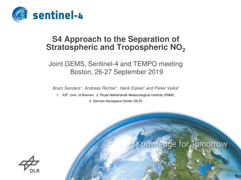
S4 Approach to the Separation of Stratospheric and Tropospheric NO2 Joint GEMS, Sentinel-4 and TEMPO meeting Boston, 26-27 September 2019 Bram Sanders1, Andreas Richter1, Henk Eskes2 and Pieter Valks3 1. IUP, Univ. of Bremen, 2. Royal Netherlands Meteorological Institute (KNMI), 3. German Aerospace Center (DLR)
Outline S4 Approach to the Separation of Stratospheric and Tropospheric NO2 S4 Approach to A-Priori Forecast Data from CAMS
Main NO2 retrieval steps Spectral retrieval of NO2slant columns using the DOAS technique 1. Separation of slant columns into a stratospheric and tropospheric part (STS) Strat. and trop. NO2are well separated Strat. NO2fields vary smoothly Trop. NO2is absent in unpolluted regions 2. Conversion of tropospheric slant columns to vertical columns using air mass factors 3.
STS: Two different approaches Baseline approach for S4: Stratospheric forecast from a global model using a data assimilation approach Implemented in operational KNMI NO2processor for S5P Alternative approach: Application of a spatial filtering technique Using clean (stratosphere-dominated) slant columns NASA NO2processor for OMI (Bucsela et al., 2013) Background trop. NO2from CTM STREAM (Beirle et al. 2016) Using cloudy measurements (strat. NO2only) To be implemented in the operational GOME-2 NO2processor
STS: challenges for geostationary sensors Applying model forecast with data assimilation is challenging for S4 1. Only small part of the globe is observed by S4 Problem if only S4 slant columns are assimilated Stratospheric model bias from unconstrained part (outside S4 domain) will be transported into S4 domain Limited number of unpolluted pixels in S4 domain 2. S4 samples the diurnal variability Diurnal variability in strat. NO2needs to be accounted for 3.
STS: Baseline approach for S4 Operational algorithm: Stratospheric forecast from CAMS global analysis system Assimilation NO2observations from polar orbiting satellites (S5P, S5) possibly also assimilation of S4 NO2observations Bias correction for inter-instrument offsets needed Comparison with S4 observations over clean and cloudy regions Bread-board algorithm: Stratospheric forecast from TM5 model (KNMI) Assimilation of S5P NO2columns
S4 STS: Bread-board algorithm Stratospheric NO2columns calculated with TM5 Horizontal resolution: 1 by 1 34 vertical model layers Output time step: 1 hour (or 30 min.) Assimilation of S5P slant columns Kalman filter technique Observations over clean and cloudy regions have large weight Strat. chemistry of model in agreement with observations Spatial and temporal bias correction needed Inter-instrument biases between S5P and S4 Diurnal variability not sufficiently constrained by S5P assimilation Alternative: assimilation of S4 slant columns
S4 STS: Operational algorithm Stratospheric NO2columns from the CAMS global analysis system Current operational CAMS global system: IFS-CB05 60 vertical model layers Horizontal resolution: 40 x 40 km 4D-Var assimilation scheme No stratospheric NOxchemistry scheme Output time step: 3 hours Advanced IFS system (Huijnen et al., 2016, 2019) IFS-CBA 137 vertical model layers Strat. chemistry scheme from the BASCOE system Output time step: 1 hour
Diurnal variation of the strat. NO2column Sampling of modelled stratospheric NO2 vertical column NO2 Vertical Column [1015 molec cm-2] 6 high resolution model three hourly sampling a three hourly sampling b three hourly sampling c 5 4 3 2 1 0 04:00 06:00 08:00 10:00 12:00 14:00 16:00 18:00 Vienna 27 September 2014
S4 Approach to a-priori Forecast Data from CAMS Joint GEMS, Sentinel-4 and TEMPO meeting Boston, 26-27 September 2019 Bram Sanders1, J. Van Gent2, Andreas Richter1, Henk Eskes3 and Pieter Valks4 1. IUP, Univ. of Bremen, 2. Belgian Institute for Space Aeronomy (BIRA-IASB), 3. Royal Netherlands Meteorological Institute (KNMI), 4. German Aerospace Center (DLR)
Use of model data Retrievals of NO2,SO2, HCHO, CHOCHO and O3use model data A priori concentration profiles Meteorological fields Horizontal spatial resolution of S4: ~8 km A priori data from coarse-resolution global models not optimal Operational forecast models that assimilate available satellite data Integrated Forecast System (IFS) of CAMS-Global (strat+trop) CAMS regional model ensemble (trop)
Use of meteorological model data Meteorological fields needed Temperature profile Surface pressure Tropopause pressure Specific humidity (pressure-height conversion) Boundary layer height Wind speed/direction CAMS-Global or ECMWF NWP stream
CAMS-Global: current situation IFS - Global atmospheric composition forecasting and data assimilation system Current operational CAMS global system: IFS-CB05 60 vertical model layers (sigma-pressure coordinates) Horizontal resolution: 40 x 40 km (reduced Gaussian grid N256) NO2, SO2, HCHO and O3fields Aerosols: AOT and mass mixing ratio profiles 4D-Var assimilation scheme No stratospheric NOxchemistry scheme Forecast base times: 0h UTC and 12 h UTC Forecast length: 5 days Output time step: 3 hours
CAMS-Global: S4 model needs Output time step 1h Stratospheric NOxchemistry (e.g. IFC-CBA) Diurnal cycle Vertical profiles Assimilation of total NO2columns from polar orbiters (S5P) CHOCHO chemistry and output (e.g. IFC-CBA)
CAMS regional model ensemble Ensemble product: median of 7 regional AQ models Region: 25 W - 45 E and 30 -70 N 8 vertical model layers (0 - 5000 m) Horizontal resolution: 0.1 x 0.1 Output species: CO, NH3, NO, NO2, SO2, O3,NMVOC, PAN Aerosols: PM2.5 & PM10 (mass conc. profiles) Output time step: 1 h S4 model needs HCHO and CHOCHO profile output Aerosol mass absorption and scattering coefficients
Merging CAMS global and regional models 1. Interpolate regional profile of mixing ratios onto the vertical grid of the global profile. Use the vertical grid of global model as common grid 2. The merged profile is the weighted average per layer of the global and regional mixing ratio profiles. Weight factor of the regional profile: - layers between surface and top of boundary layer weight one - highest common layer around 5 km weight zero - layers between boundary layer and 5 km linear interpolation
Spatial resolution: Copenhagen Underestimation of NO2and SO2by the global model pollution hotspot effect of horizontal spatial resolution
Spatial resolution: English Channel overestimation of NO2and SO2by the global model outflow region
Free troposphere: North Atlantic Global NO2and SO2 profiles have features in the free troposphere that are not present in the regional model. The regional models are air quality models: Less accurate chemistry schemes for the free troposphere in the regional models. Vertical grid of ensemble median is coarse in free troposphere.
ECMWF-CAMS (ECA) pre-processor ECA processor delivers meteorological and chemical variables for the time and geolocation of the L1b pixel. On pixel grids for the UVis and NIR channels separately, as needed. The ECA processor ingests operational model data from ECMWF, CAMS Global and CAMS Regional as they come. The processor is flexible with respect to improvements in horizontal resolution, vertical layering and time step.
ECA processor: dynamic input Forecast variable Short name Unit Source ECMWF CAMS Global CAMS Regional t q sp K kg kg-1 Pa x x x missing x x x +Temperature +Specific humidity Surface pressure Tropopause pressure ? Boundary layer height 10-m U wind component 10-m V wind component +NO2mixing ratio +SO2mixing ratio blh 10u 10v no2 so2 m m s-1 m s-1 kg kg-1 kg kg-1 x x hcho go3 kg kg-1 kg kg-1 kg kg-1 x missing x +HCHO mixing ratio +CHOCHO mixing ratio +O3mixing ratio ( GEMS Ozone ) +Sea salt (0.03 - 0.5 m) mixing ratio +Sea salt (0.5 - 5 m) mixing ratio +Sea salt (5 - 20 m) mixing ratio +Dust (0.03 - 0.55 m) mixing ratio +Dust (0.55 - 0.9 m) mixing ratio +Dust (0.9 - 20 m) mixing ratio +Hydrophobic organic matter mixing ratio +Hydrophilic organic matter mixing ratio +Hydrophobic black carbon mixing ratio +Hydrophilic black carbon mixing ratio +Sulphate aerosol mixing ratio +NO2concentration +SO2concentration +HCHO concentration +CHOCHO concentration +O3concentration aermr01 aermr02 aermr03 aermr04 aermr05 aermr06 aermr07 kg kg-1 kg kg-1 kg kg-1 kg kg-1 kg kg-1 kg kg-1 kg kg-1 x x x x x x x aermr08 kg kg-1 x aermr09 kg kg-1 x aermr10 aermr11 no2_conc so2_conc kg kg-1 kg kg-1 g m-3 g m-3 g m-3 g m-3 g m-3 x x x x missing missing x o3_conc
ECA processor: output Variable name Unit Comment Type Dims. L2 core processor NO2 SO2 HCH CH OTO OTR CLD ALH UAI SUR O x K K kg kg-1 f32 f32 f32 g x s x l g x s x l g x s x l x x x x x x temperature_uvvis temperature_nir specific_humidity_uvvis x x kg kg-1 f32 g x s x l specific_humidity_nir m terrain-corrected, PSF- weighted average elevation; pixel elevation copied from L1b f32 g x s [pixel elevation on uvvis: name from L1b] m f32 f32 g x s g x s [pixel elevation on nir: name from L1b] [pixel observation times on uvis, name from L1b] only times for UVis channel; copied from L1b nominal geolocation reported in ECA files for easy visualisation; copied from L1b f32 g x s [nominal latitude on uvvis; name from L1b] f32 g x s [nominal longitude on uvvis; name from L1b] f32 g x s [nominal latitude on nir; name from L1b] f32 g x s [nominal longitude on nir; name from L1b] Pa Pa - f32 f32 ui16 g x s g x s g x s x x x x x x x surface_pressure_uvvis surface_pressure_nir tropopause_layer_index_uvvis x x index of uppermost layer assigned to troposphere (???) height a.g.l. U component x x x x m m s-1 f32 f32 g x s g x s x x x x x x x x boundary_layer_height_uvvis eastward_wind_at_10m_uvvis m s-1 V component f32 g x s x x x x northward_wind_at_10m_uvvis mol m-2 f32 g x s x l x nitrogendioxide_partial_columns_uvvis mol m-2 f32 g x s x l x sulfurdioxide_partial_columns_uvvis mol m-2 f32 g x s x l x formaldehyde_partial_columns_uvvis mol m-2 f32 g x s x l x glyoxal_partial_columns_uvvis mol m-2 f32 g x s x l x x x ozone_partial_columns_uvvis f32 f32 g x s x l g x s x l x x x x x x x x aerosol_volume_absorption_coefficient aerosol_volume_scattering_coefficient


 pre-processor")