Real-time Monitoring in Dynamic Sensor Networks: LiMoSense Study

This study delves into LiMoSense, a live monitoring approach for dynamic sensor networks, exploring challenges such as correctness, convergence, and dynamic behavior. The research focuses on sensors' communication, aggregation of read values, and the use of bidirectional and unidirectional communication for error-free aggregation. The study also discusses the realism of monitoring in dynamic inputs and the constraints posed by cheap sensors and limited batteries.

• Sensor Networks
• Real-time Monitoring
• Dynamic Behavior
• Error-Free Aggregation
• LiMoSense

byru_yar Follow

Uploaded on Oct 03, 2024 | 0 Views

Download Presentation

Please find below an Image/Link to download the presentation.

The content on the website is provided AS IS for your information and personal use only. It may not be sold, licensed, or shared on other websites without obtaining consent from the author. Download presentation by click this link. If you encounter any issues during the download, it is possible that the publisher has removed the file from their server.

Presentation Transcript

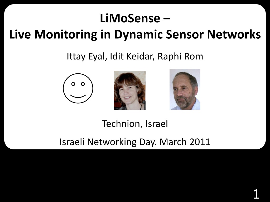
1. LiMoSense Live Monitoring in Dynamic Sensor Networks Ittay Eyal, Idit Keidar, Raphi Rom Technion, Israel Israeli Networking Day. March 2011 1

2. Outline Background static average aggregation in sensor networks. LiMoSense. Correctness. Convergence. Dynamic behavior. 2

3. Sensors Read values and communicate. Light-weight, little energy, error prone. 3

4. Sensor Network Many sensors (at least thousands). Limited topology. Similar scenario in cloud monitoring 4

5. Average Aggregation Target: Average of read values. Reason: Environmental monitoring. Cloud computing load monitoring. Challenge: Cannot collect the values. Solution: In-network aggregation. Hierarchical solution? Not robust. 5

6. Static error-free aggregation [1,2] Bidirectional communication gossip 8 5 5 3 3 4 2 5 4 t=1 t=2 t=3 1. 2. D. Kempe, A. Dobra, and J. Gehrke. Gossip-based computation of aggregate information. In FOCS, 2003. S. Nath, P. B. Gibbons, S. Seshan, and Z. R. Anderson. Synopsis diffusion for robust aggregation in sensor networks. In SenSys, 2004. 6

7. Static error-free aggregation [1,2] Unidirectional communication gossip v w ( A v Send half: 2, ) w 1 3, 1 3, 0.5 A (3, 0.5) A + + w v in in w v w = B B v B w in B 5, 1 4.3, 1.5 B 1. 2. D. Kempe, A. Dobra, and J. Gehrke. Gossip-based computation of aggregate information. In FOCS, 2003. S. Nath, P. B. Gibbons, S. Seshan, and Z. R. Anderson. Synopsis diffusion for robust aggregation in sensor networks. In SenSys, 2004. 7

8. Static error-free aggregation [1,2] Unidirectional communication gossip v w 4, x 3, 1 A (3, 0.5) t 4, y 5, 1 B 1. 2. D. Kempe, A. Dobra, and J. Gehrke. Gossip-based computation of aggregate information. In FOCS, 2003. S. Nath, P. B. Gibbons, S. Seshan, and Z. R. Anderson. Synopsis diffusion for robust aggregation in sensor networks. In SenSys, 2004. 8

9. Static error-free aggregation Realistic? Monitoring Dynamic input! (restart?) Cheap sensors Crashes. Limited battery Link failure and message loss 9

10. LiMoSense Live Monitoring in Dynamic Sensor Networks 10

11. Live error-free aggregation Observation: Invariant: read sum = Weighted sum 3, 1 3, 1/2 A 3 1 5 1 8 + = 3 1/ 2 + 4.3 3/ 2 = 8 5, 1 4.3, 3/2 B 11

12. Live error-free aggregation Observation: Invariant: read sum = Weighted sum Goal: Maintain the invariant after input changes. 12

13. Live error-free aggregation Each node stores: 1. Current weighted value. 2. Previously read value. On read change: update weighted value to fix invariant. 1 newRead i i i w Weight unchanged. ( ) + prevRead est est i i 13

14. Live error-free aggregation 1 w ( ) + newRead prevRead est est i i i i i Example: read value 0 1 3, 1 3, 2 Before 4, 1 3.5, 2 After Case 1: Case 2: 14

15. Live robust aggregation Lost messages lost weight broken Invariant: 3, 1 3, 0.5 (3, 0.5) (3, 0.25) 15

16. Live robust aggregation Solution: Send summary, not diff: 3, 1 3, 0.5 3, 1 3, 0.5 (3, 0.5) (3, 0.5) (3, 0.25) (3, 0.75) 16

17. Live robust aggregation Solution: Send summary, not diff: Lost message: Fix on next one. Failed link: Transfer undo. 3, 1 3, 0.5 (3, 0.5) (3, 0.75) 17

18. Live robust aggregation Solution: Send summary, not diff: 3, 1 3, 0.5 3, 0.25 3, 1 (3, 0.5) Undo (3, 0.75) Link fail 18

19. Live robust aggregation Challenge: weight infinity Solution: Hybrid push-pull: Ask neighbor to send back inverse. 3, 1 3, 0.5 (3, 0.75) (3, 0.5) 19

20. Live robust aggregation Challenge: weight infinity Solution: Hybrid push-pull: Ask neighbor to send back inverse. 3, 1 3, 0.5 (3, -0.5) pull (3, 0.5) 20

21. Live robust aggregation Crashed node lost links. 21

22. Correctness Correctness 22

23. Correctness - Safety Theorem 1: The invariant always holds. 1. On message send/receive. 2. After value change. 3. After add/remove neighbor. 4. After node removal/addition. 23

24. Correctness - Liveness Theorem 2: After GST, all estimations converge to the average. 1. Quantization constant and fairness. 2. Value propagation. 3. Convergence. 24

25. Correctness - Liveness 1. Quantization constant and fairness. Weight is transferred in multiples of q. Note This does not effect accuracy. Each node eventually succeeds to send a push message to all of its neighbors. 25

26. Correctness - Liveness 2. Value propagation. Lemma: For any time t >= GST and node i, there exists a time t > t after which every node j has a component of i with a weight larger than some bound (the bound is dependent on n and q) 26

27. 27

28. Correctness - Liveness 3. Convergence. Define a series GST =t0, t1, t2, ... Where at ti each node has a bounded- from-below portion from each node at ti-1. At each ti, the largest error is smaller than in ti-1, because it's mixed with other values. 28

29. Convergence Rate Convergence Rate 29

30. Convergence Static convergence rate (exchange gossip): Static input (after GST). Dense topology. Synchronous uniform runs. 30

31. Convergence Static convergence rate (exchange gossip): Assumption: normal distribution of estimations. 31

32. Convergence Static convergence rate (exchange gossip): 32

33. Simulation Simulation 33

34. Step Function 100 nodes. Standard Normal distribution 10 nodes change Values (+10) 34

35. Step Function 100 nodes. Standard Normal distribution 10 nodes change Values (+10) 35

36. Step Function 100 nodes. Standard Normal distribution 10 nodes change Values (+10) 36

37. Creeping Value Change 100 nodes. Standard Normal distribution Every 10 steps, 10 nodes change Values (+0.01) 37

38. Creeping Value Change 100 nodes. Standard Normal distribution Every 10 steps, 10 nodes change Values (+0.01) 38

39. Creeping Value Change 100 nodes. Standard Normal distribution Every 10 steps, 10 nodes change Values (+0.01) 39

40. Response to Step Function 100 nodes. Standard Normal distribution 10 nodes change Values (+10) for 100 steps 40

41. Response to Step Function 100 nodes. Standard Normal distribution 10 nodes change Values (+10) for 100 steps 41

42. Dynamic Network Disc Graph t=2500: 10 nodes range decay, 7 lost links t=5000: Node crash. 42

43. Summary LiMoSense Live Average Monitoring in error prone dynamic sensor networks. Live: aggregate dynamic data reads. Fault tolerant: Message loss, link failure and node crash. Correctness in dynamic asynchronous settings. Exponential convergence after GST. Quick dynamic behavior. Ittay Eyal, Idit Keidar, Raphael Rom. LiMoSense - Live Monitoring in Dynamic Sensor Networks, Technion technical report CCIT #786 March 2011EE. 43

44. Good Questions Good Questions 44

45. Convergence Static convergence rate (push gossip): 45