Understanding Models with False Positive Detections in Occupancy Modeling
Explore the importance of addressing false positives in occupancy modeling, potential biases caused by them, methods to mitigate errors, and the extension of basic occupancy models to allow for false positives. Key concepts such as the Royle-Link model and the integration of classification processes with ecological models are discussed, highlighting the complexities and considerations in ecological data analysis.
Download Presentation
Please find below an Image/Link to download the presentation.
The content on the website is provided AS IS for your information and personal use only. It may not be sold, licensed, or shared on other websites without obtaining consent from the author. Download presentation by click this link. If you encounter any issues during the download, it is possible that the publisher has removed the file from their server.

Presentation Transcript
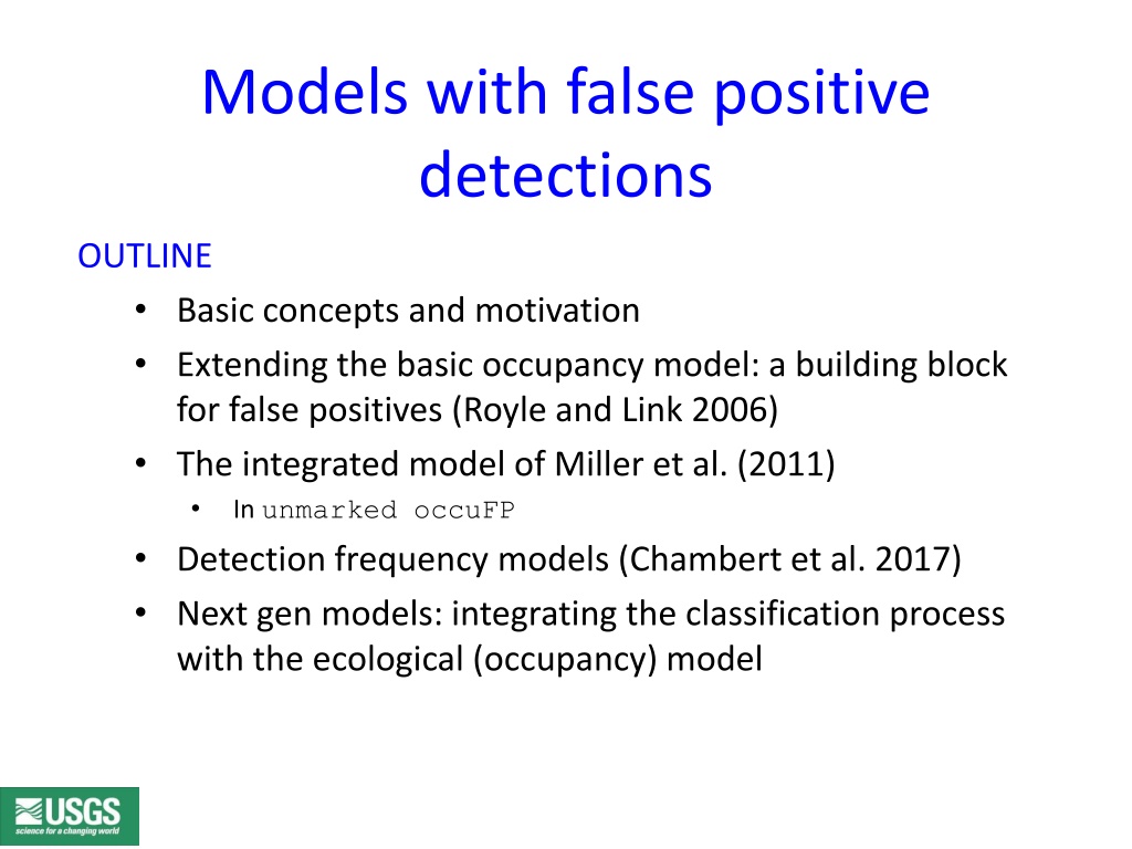
Models with false positive detections OUTLINE Basic concepts and motivation Extending the basic occupancy model: a building block for false positives (Royle and Link 2006) The integrated model of Miller et al. (2011) In unmarked occuFP Detection frequency models (Chambert et al. 2017) Next gen models: integrating the classification process with the ecological (occupancy) model
Models with false positive detections A basic occupancy model assumes that there are no false positives. A detection is a valid detection (i.e., y = 1 means the species occurs with certainty!) This can be incorrect. E.g., observers are highly variable in skill level (e.g., imagine citizen science schemes) and thus errors can be made Contemporary context: New technologies that are interpreted automatically (ML/AI) produce errors! Acoustic monitoring Camera trapping eDNA
False positives Why do we care? Even small rates of false positives produce large bias in parameter estimates. Unfortunate property of sampling with false positives: ? 1 as ????? increases Therefore, attempts should be made to address FPs Conservative thinning threshold (e.g., PID in genetics) Expert validation of detections Models that allow false positives!
A basic model The traditional occupancy model ?? ???? ? ?? This implies no false positives. Effective detection probability = 0 if ? = 0 Extension to allow false positives: ?? ????(? ??+ ??? 1 ??) Interpretation: if a site is occupied you detect the species with probability ? but if a site is unoccupied you detect the species with probability ??? Royle and Link (Ecology, 2006)
Royle-Link model You can estimate both ? and ??? from ordinary occupancy data with an important caveat (see next) But note: it is a model of site classification not a model of sample classification so it is not exactly coherent with respect to how surveys are done (which record sample level data and aggregate those up to the site) How do you scale sample level detections up to the site level? (we talk about this later)
The caveat: multi-modality This observation model allowing for false positives is precisely a finite mixture model such as the type of model that was made popular in ecological statistics by Norris and Pollock (1996), Pledger (2000), and others for modeling detection heterogeneity in capture-recapture models. A well-known feature of such models is that the likelihood is inherently multi-modal (i.e., does not have a unique solution). The likelihood for the parameter values (?, ???,?) is the same as ???, ?,1 ? This gets really, really complicated in multiple dimensions! (with > 2 classes). Imagine a CT study with 20 species, or acoustic monitoring study with 100 species of birds.
The caveat: multi-modality One solution to this is to impose a sensible constraint: ?11> ?10 i.e., the probability of detecting the species at an occupied site is greater than an unoccupied site (embarrassingly we wrote this wrongly in the chapter!). Constraints become complicated when there are > 2 classes! As such, it is especially important to control for extraneous heterogeneity in detection when false positives are of direct interest. In other words, unmodeled heterogeneity can look like false positives and vice versa. Fitzpatrick et al. (2009) provide an illustration of this phenomenon (heterogeneity due to variable abundance of an invasive insect). The other way to deal with multi-modality is to have some perfect information (Miller et al. 2011). i.e., validation data.
R template: simulation and model fitting when you have data contaminated with false positives # Build the unmarkedFrame summary(umf <- unmarkedFrameOccuFP(y = y, type = type)) # not shown umf.occ<- unmarkedFrameOccu(y=y) # These starting values are consistent with our preferred constraint largerp10 <- qlogis(c(0.5, 0.1, 0.7)) # Order is psi, p, fp # Using these starting values will find the wrong mode. largerp11 <- qlogis(c(0.5, 0.7, 0.1)) # Fit the model (m1 <- occuFP(detformula = ~1, # model for p_11 FPformula = ~1, # model for p_10 stateformula = ~1, # model for psi data = umf, # umarkedFrameOccuFP object starts = largerp11) ) # add p_10 < p_11 constraint
Millers multi-state model A general modeling framework that integrates data of 3 different types: Type 1 data: ordinary occupancy data, false negatives but no false positives Type 2 data: ordinary occupancy data, but contaminated with random false positives (i.e., Royle-Link) Type 3 data: Positive observations are a mix of uncertain positives and confirmed positives. So, there is some confirmation mechanism going on behind the curtain. They describe an integrated, multi-state model for data that are a mix of these different types.
Type 3 data For Type 3 data we code the observations as 0, 1 or 2 (by convention) 0 = not detected 1 = uncertain detection (could be FP). E.g., scat or sign, citizen sighting 2 = certain detection (true positive). E.g., visual or trained expert. Values of 2 arise by some confirmation mechanism by which a subset of sites where detections occurred become confirmed positives
Type 3 data Type 3 data have a multinomial likelihood conditional on ? ? = probability an occupied site where detection occurs gets confirmed
Occupancy models w/false-positives in unmarked unmarked has a very versatile function for fitting these models. It allows for a mix of all 3 types of data: occuFP(detformula = ~1, FPformula = ~1, Bformula = ~1, stateformula = ~1, data, starts ) Bformula: sites may vary in their likelihood of being confirmed. Miller et al. used high calling intensity to define the certain state and related b to air temperature. (p was also related to air temperature .) Note: starts are not in formula order! Starting values order is: psi, p, fp, b (sometimes you have to read the R code to deduce this).
Fitting the Miller et al. model in unmarked You have to declare the type of data. The unmarkedFrame constructor function has a type argument. Suppose you just have Type 2 data (occupancy data contaminated with false positives, no confirmation) for ? = 7 survey occasions type <- c(0, 7, 0) umf <- unmarkedFrameOccuFP(y = y, type = type) Suppose the first 2 periods are Type 1 data (expert listened to all the audio files) type <- c(2, 5, 0) Suppose the 7th period involved visiting some sites with a human observer to confirm type <- c(2, 4, 1)
Miller et al. model comments Confirmation is a site level process, the mechanism by which individual samples within a site are confirmed or not is not specified. But in practice we know that false positives at the site level happen by making (incorrect) sample-level classifications. Model structure is that of a Bernoulli confirmation process for all sites. Implies that all sites have a chance at confirmation. The number confirmed is a random variable. If a site has a detection that may be confirmed, couldn t it be confirmed negative also? E.g., if you re using DNA as the confirmation method NO! Confirmation of a sample is sufficient to confirm presence, but confirmation that the sample is non target does not confirm the site is unoccupied.
Work session (see R script) I m going to go over the most general example here, that which involves all 3 data types (this is Part 3 in the script)
# Simulation settings set.seed(2019) # RNG seed nsites <- 200 # number of sites nsurveys <- 7 # number of occasions habitat <- rnorm(nsites) # Some (continuous) habitat descriptor # Simulate the occupancy states and data alpha0 <- 0 # Intercept... alpha1 <- 1 # ... and slope of psi-habitat regression psi <- plogis(alpha0 + alpha1*habitat) # Occupancy z <- rbinom(nsites, 1, psi) # Latent p/a states y <- matrix(0,nsites, nsurveys) p <- c(0.7, 0.5) # method 2 will have a lower p b <- 0.5 # probability that observed positive is confirmed certain fp <- 0.05 # False-positive prob.
# Simulate data of all 3 types. Note p differs between occ 1-2 and 3-7. # False positives occur in occasions 3-7 but in occasion 7 there are some confirmed positives for(i in 1:nsites){ # Normal occupancy data y[i, 1:2] <- rbinom(2, 1, p[1]*z[i]) # False-positives mixed in y[i, 3:6] <- rbinom(4, 1, p[2]*z[i] + fp*(1-z[i])) # Type 3 observations are occupancy data contaminated with false positives but then # we identify some of them as true (after the loop closes) y[i, 7] <- rbinom(1, 1, p[2]*z[i] + fp*(1-z[i])) } # Here we set some of the detections to confirmed positives true.positives <- z==1 & y[,7]==1 confirmed <- (rbinom(nsites, 1, b) == 1) & true.positives y[confirmed, 7] <- 2
# Make a covariate to distinguish between the two methods Method <- matrix(c(rep("1", 2), rep("2", 5)), nrow = nsites, ncol = 7, byrow = TRUE) # Type indicates a mix of all 3 data types type <- c(2, 4, 1) # Same covariate structure as before siteCovs <- data.frame(habitat = habitat) obsCovs <- list(Method = Method) summary(umf1 <- unmarkedFrameOccuFP(y, siteCovs = siteCovs, obsCovs = obsCovs, type = type)) # fp starting value should be small (-1 here). # Note: last parameter in this model is "Pcertain" ( m3 <- occuFP(detformula = ~ -1 + Method, FPformula = ~1, Bformula = ~1, stateformula = ~ habitat, data = umf1, starts=c(0, 0, 0, 0, -1, 0)) ) # starting values order: psi parms, p parms, fp parms, b parms.
Call: occuFP(detformula = ~-1 + Method, FPformula = ~1, Bformula = ~1, stateformula = ~habitat, data = umf1, starts = c(0, 0, 0, 0, 0, -1)) Occupancy: Estimate SE z P(>|z|) (Intercept) -0.0813 0.160 -0.509 6.11e-01 habitat 0.9495 0.198 4.791 1.66e-06 Detection: Estimate SE z P(>|z|) Method1 0.9751 0.1802 5.412 6.22e-08 Method2 0.0155 0.0954 0.163 8.71e-01 false positive: Estimate SE z P(>|z|) -2.86 0.207 -13.8 1.29e-43 Remember: estimates are on the logit scale for probability parameters Pcertain: Estimate SE z P(>|z|) 0.0388 0.292 0.133 0.894 AIC: 1383.091
A bit of Bayesian analysis FP models, including multi-state model, can be written out directly in the BUGS language Initial values are really important! Try to start p and fp near the correct mode (p > fp)
Example of a multi-method model. Ordinary occupancy data + Site-confirmation data # Specify model in BUGS language cat(file = "occufp2.txt"," model { # Priors psi ~ dunif(0, 1) fp ~ dunif(0, 1) b ~ dunif(0, 1) alpha0 ~ dnorm(0,0.01) alpha1 ~ dnorm(0,0.01) # Method effect # Likelihood and process model for (i in 1:nsites) { # Loop over sites z[i] ~ dbern(psi) # State model # Define observation matrix (obsmat) for(j in 1:(nsurv1+nsurv2)) { obsmat[i,j,1,1] <- 1-fp # z = 0 obs probs obsmat[i,j,2,1] <- fp obsmat[i,j,3,1] <- 0 obsmat[i,j,1,2] <- 1-p[i,j] # z = 1 obs probs obsmat[i,j,2,2] <- (1-b)*p[i,j] obsmat[i,j,3,2] <- p[i,j]*b } # Observation model: part 1 (for first 3 cols in y) for(j in 1:nsurv1) { # Loop over replicate surveys logit(p[i,j]) <- alpha0 y[i,j] ~ dbern(z[i]*p[i,j] ) # ordinary occupancy data } # Observation model: Type 3 data (for last 4 cols in y) for (j in (nsurv1+1):(nsurv1+nsurv2)) { logit(p[i,j]) <- alpha0 + alpha1 y[i,j] ~ dcat(obsmat[i,j,1:3,z[i]+1] ) } } } ") Build the observation state probability matrix here This is the new part compared to an ordinary occupancy model
Sample-level models for false positives Site-level classification: Real world doesn t work that way! Most methods produce a stochastic number of samples for a site: camera traps, ARUs, human observers. Errors in classification (i.e., false positives) occur at the sample level. We would like an occupancy model that accommodates sample level data and misclassification, so that your inference about site classification properly scales with the number and quality of samples produced
Machine learning pipeline ??,?= frequency of putative targets Machine learning algorithm ML/AI methods produce false positives! Model proposed by Chambert et al. 2017:
Sample-level models for false positives Conceptual model for observed data: ??,?= actual targets (true positives) + misclassifications (false positives) A natural model for contaminated data: ??,? ??????? ? ??+ ? ?? ???? ?? Target producing mechanism and non-target mechanism have to be independent! ? = mean number of target detections per site ??= occupancy status at site ? ? = mean number of false-positives per site You observe a count with expected value ? if the species is not present and ? + ? if the species is present. This is a natural sample-frequency version of the false positives occupancy model.
Sample-level models for false positives Integrated models: Could imagine other data sources provide information about ?, independent of the detection frequencies. E.g., suppose detection frequencies are generated by ARUs and machine learning which is producing false positives, and your highly trained field observers are producing normal occupancy data. i.e., a 2nd data source: ???? ? ?? ??,? Or with false positives
Implementation in JAGS This model does not exist in unmarked (but would be easy to do .) We show a brief simulation of the integrated model (contaminated occupancy + contaminated detection frequencies)
# Simulation settings set.seed(2019, kind = "Mersenne") nsites <- 100 # Number of sites nsurveys <- 5 # Number of replicates/occasions psi <- 0.7 # Occupancy p11 <- 0.5 # Detection probability at an occupied site p10 <- 0.05 # False detection probability lam <- 3 # Rate of true positives from ARU ome <- 0.50 # Rate of false positives from ARU # Simulate true occupancy states z <- rbinom(nsites, 1, psi) # Define detection probability p <- z * p11 + (1-z) * p10 # Simulate occupancy data and ARU count frequencies yARU <- y <- K <- Q <- matrix(NA, nsites, nsurveys) for(i in 1:nsites){ y[i,] <- rbinom(nsurveys, 1, p[i]) # Detection/nondetection data K[i,] <- rpois(nsurveys, lam*z[i]) # True positive detection frequency Q[i,] <- rpois(nsurveys, ome) # False-positive detection frequency yARU[i,] <- K[i,] + Q[i,] # Number of ARU detections } # Bundle and summarize data str( bdata <- list(y = y, yARU = yARU, nsites = nsites, nsurveys = nsurveys ))
# Specify Model A in BUGS language cat(file = "modelA.txt"," model { # Priors psi ~ dunif(0, 1) # psi = Pr(Occupancy) p10 ~ dunif(0, 1) # p10 = Pr(y = 1 | z = 0) p11 ~ dunif(0, 1) # p11 = Pr(y = 1 | z = 1) lam ~ dunif(0, 1000) ome ~ dunif(0, 1000) # Likelihood:process and observation models for (i in 1:nsites) { z[i] ~ dbern(psi) # Occupancy status of site i p[i] <- z[i] * p11 + (1-z[i]) * p10 # false-positive detection model for(j in 1:nsurveys) { y[i,j] ~ dbern(p[i]) # Binary occupancy data yARU[i,j] ~ dpois(lam * z[i] + ome) # ARU detection frequency data } } } ") # Initial values inits <- function(){list(z = apply(y, 1, max), psi = runif(1), p10 = runif(1, 0, 0.05), p11 = runif(1, 0.5, 0.8), lam = runif(1, 1, 2), ome = runif(1, 0, 0.4) )} # Parameters monitored params <- c("psi", "p10", "p11", "lam", "ome") # MCMC settings na <- 1000 ; ni <- 2000 ; nt <- 1 ; nb <- 1000 ; nc <- 3 # Call JAGS (tiny ART), gauge convergence and summarize posteriors out1 <- jags(bdata, inits, params, "modelA.txt", n.adapt = na, n.chains = nc, n.thin = nt, n.iter = ni, n.burnin = nb, parallel = TRUE) par(mfrow = c(2, 3)) ; traceplot(out1) print(out1, 3) This model has contaminated occupancy data and contaminated detection frequency data such as from an ARU
Validation data Usually (in a ML workflow) there is some level of expert validation. We would like to use this information to inform model parameters. Suppose a batch of detections contains ? true positives, ? false positives, you choose ? samples to validate of which ? turn out to be correctly classified.Then,? has a hypergeometric distribution ? ? ???? ?,?,?,1 In practice we do this by site and so ?? are input as data to JAGS, and the model is expanded to include the hypergeometric likelihood of these data. Standard model for sampling without replacement.
Next gen models The detection frequency model assumes that each detection is classified somehow. i.e., a computer algorithm is declaring detected signals to be targets. In practice there is usually some additional information that the algorithm is using to decide which detections are (most likely) the target. And the amount of information varies from sample to sample. Thus, there is heterogeneity in classification accuracy that is sample-specific E.g., match scores in acoustic data processing Feature score vector produced by a CNN How can we use this information in occupancy models?
Next gen models ??,?= frequency of putative targets Machine learning algorithm ML/AI methods produce false positives! In practice, detection frequencies ? are treated as observed quantities but they are aggregations of detections which are estimates of true latent class , and estimated with variable precision by the black box . What to do about it?
Next gen models Next gen models: Integrate the classification process (and hence the uncertainty) with the ecological models (see Ch. 7 of AHM2) Sample class is itself a latent variable, not a deterministic quantity spit out of a black box Hence the classification process is part of the model High-dimensional (multi-species, community )