Evolutionary Models in Molecular Biology

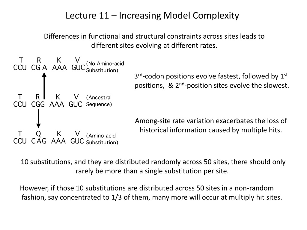
Differences in functional and structural constraints across sites lead to varying rates of evolution in molecular sequences. Understanding the complexities of site-specific rates, among-site rate variation, site-specific rates models, invariable sites model, and continuous methods is crucial for accurate phylogenetic reconstruction. These models help in capturing the evolutionary dynamics and patterns of substitution in molecular data, aiding in inferring historical relationships and estimating divergence times.

Download Presentation

Please find below an Image/Link to download the presentation.

The content on the website is provided AS IS for your information and personal use only. It may not be sold, licensed, or shared on other websites without obtaining consent from the author. Download presentation by click this link. If you encounter any issues during the download, it is possible that the publisher has removed the file from their server.

• Evolutionary Models
• Molecular Biology
• Phylogenetic Reconstruction
• Site-Specific Rates
• Substitution Patterns

gianni Follow

Uploaded on Apr 07, 2024 | 5 Views

Presentation Transcript

1. Lecture 11 Increasing Model Complexity Differences in functional and structural constraints across sites leads to different sites evolving at different rates. 3rd-codon positions evolve fastest, followed by 1st positions, & 2nd-position sites evolve the slowest. Among-site rate variation exacerbates the loss of historical information caused by multiple hits. 10 substitutions, and they are distributed randomly across 50 sites, there should only rarely be more than a single substitution per site. However, if those 10 substitutions are distributed across 50 sites in a non-random fashion, say concentrated to 1/3 of them, many more will occur at multiply hit sites.

2. Among-site rate variation Discrete methods assign sites to a series of rate categories (or partitions). Add a relative rate parameter, r,to our models. Pij(t,r) ={1/4 - 1/4 e 1/4 + 3/4 e-4art for i = j -4art for i = j c i= lnLt wrlnL(i,r) r=1 There are c rate categories, and wr is the probability that site i belongs to a particular rate category; these are binary (0 or 1) if we re assigning sites to rate classes.

3. Site-Specific Rates (or SSR) model In the SSR models, the theoretical limit to the number of rate categories is the number of sites in the alignment, but usually these are determined a priori and often they follow codon structure. So in this case, w1, w2, and w3 are fixed to 0 or 1, and we just use a different relative rate for each class (e.g., codon position). The relative rate parameters then can be assigned, or they can be optimized numerically, which is what is usually done. Advantage: one also can use a different transformation matrix (Q) for each class. Disadvantage: that all sites within a category are assumed to be evolving a uniform rate.

4. Invariable Sites Model This is based on observations that there are sites in alignments of conserved genes which all life seem to have the same state. This allows two rate categories and in one of these, the relative-rate parameter is zero. We can think about this model in two ways. Mixture model winvar = pinvar This is the probability that a site is in the class where r = 0. wvar =pvar The probability that the site is in the class where r 0. wvar = 1 - winvar Sites that are observed to vary have winvar = 0. Invariable sites pinvar is the proportion of sites across an alignment that are not free to vary. the proportion of sites that are observed constant.

5. ContinuousMethods There s no biological reason to expect rates to fall into discrete categories, and we can use rate-mixture models to deal with this. Gamma distributed rates. shape parameter (a) & scale parameter (b); mean = ab we set the mean of the G-distribution equal to 1 by constraining b = 1/a. ?

6. Discretizing the G-distribution 0.00 +-----------------------------------------------------------------------------------+ |#################################################################################### 3.00 +-----------------------------------------------------------------------------------+ 0.0 1.75 Gamma distribution with shape parameter (a) = 0.49 0.0 1.75 Cut-points and category rates for discrete G approximation with ncat (or c) = 4. ------ cut-points ------ cat lower upper rate (mean) -------------------------------------------------------------- 1 0.00000000 0.09804816 0.03191473 2 0.09804816 0.44841399 0.24666120 3 0.44841399 1.31969682 0.81435904 4 1.31969682 infinity 2.90706503 0.10 +########################################################## |############################################## 0.20 +####################################### |################################## 0.30 +############################## |########################### 0.40 +######################### |####################### 0.50 +##################### |################### 0.60 +################## |################# 0.70 +################ |############### 0.80 +############## |############# 0.90 +############# |############ 1.10 +########## 1.00 +########### |########### |########## 1.20 +######### |######### 1.30 +######### |######## 1.40 +######## |######## 1.50 +####### |####### 1.60 +####### |###### 1.70 +###### |###### 1.80 +###### |###### 1.90 +##### |##### 2.00 +##### |##### 2.10 +##### |#### 2.20 +#### |#### 2.30 +#### |#### 2.40 +#### |#### 2.50 +### |### 2.60 +### |### 2.70 +### |### 2.80 +### |### 2.90 +### |### So r1 = 0.0319, r2 = 0.2467, r3 = 0.8144, & r4 = 2.907; note these sum to 4 (=ncat). Each site has some non-zero probability of belonging to each rate class: wr is optimized for each of the c classes.

7. Discretizing the G-distribution Cut-points and category rates for dG w/ncat = 8 ------ cut-points ------ cat lower upper rate (mean) --------------------------------------------------------------- 1 0.00000000 0.02338747 0.00768838 2 0.02338747 0.09804816 0.05614108 3 0.09804816 0.23352213 0.16013076 4 0.23352213 0.44841399 0.33319164 5 0.44841399 0.78071211 0.60229167 6 0.78071211 1.31969682 1.02642641 7 1.31969682 2.35886822 1.77009489 8 2.35886822 infinity 4.04403517 The more highly we discretize the G, the shorter the runs, but: 0.16 0.15 0.14 Poor estimates of a with ncat < 12 a 0.13 0.12 0.11 0.1 0.09 0.08 4 6 8 10 12 14 ncat 16 18 20 22 24

8. Properties of G models This is done across the entire data set, so essentially, we take the same transformation matrix (Q) for each site and scale it by the average rate for each category. This has the large advantage of being able to accommodate such a high diversity of rates with just a single parameter, a. Some sites can be so slowly evolving to have a high probability of stasis, yet others (perhaps adjacent) may be free to evolve rapidly. It has the disadvantage that we apply the same transformation matrix uniformly across a data set one set of base frequencies and one R matrix. We may get a much better fit if we allow very different Q matrices. Furthermore, SSLs for each site are calculated many times (ncat times), so the better we approximate a continuous G, the longer our run times. It s important to note that this is actually a rather constrained mixture model.

9. I+G Models This is intuitively very appealing when one considers that, at least from some genes, there s a set of sites that are constant across essentially the tree of life. pinvar pinvar= 0 I+G = G a= G - shape parameter (a) I+G = I pinvar= 0 & a= I+G = ER Rate of Evolution There are some issues with it that are sometimes not appreciated.

10. I+G Models First, both the mixed model and the gamma alone expect there to be many constant sites. It can be very difficult to discern the sites that are truly invariable from those potentially variable sites that are evolving slowly enough to have a high probability of stasis

11. The GTR+I+G family of models There are 1624 possible special cases of GTR+I+G There are 10 parameters in the full model: 3 free b.f. (p p) 5 relative rates (R) 2 A-SRV parameters (pinvar & a) } = Q From Sullivan (2005. Methods in Enzymology, 395:757)

12. Another look at a GTR+SSR3 pA1 pC1 pG1 pT1 r(AC)1 r(AG)1 r(AT)1 r(CG)1 r(CT)1 r(GT)1 pA2 pC2 pG2 pT2 r(AC)2 r(AG)2 r(AT)2 r(CG)2 r(CT)2 r(GT)2 pA3 pC3 pG3 pT3 r(AC)3 r(AG)3 r(AT)3 r(CG)3 r(CT)3 r(GT)3 9 free base frequencies 15 relative rate parameters pA1 = pA2 = pC1 = pC2 pG1 = pG2 = pT1 = pT2 r(AC)1 = r(AC)2 = r(AG)1 =r(AG)2 = r(AT)1 =r(AT)2 = r(CG)1 =r(CG)2 = r(CT)1 =r(CT)2 = r(GT)1 =r(GT)2 = pA3 pC3 pG3 pT3 r(AC)1 r(AG)3 r(AT)3 r(CG)3 r(CT)3 r(GT)3 = = Single GTR

13. GTR+CAT in RAxML/FreeRates in IQ-TREE Estimate relative rates for each site on a starting tree. Step 1: estimate the relative rate at each site in the alignment Lump sites with similar relative rates into categories. C A A C C T G G C G T T C C A C C T G A A G A A G C A G . . . . . A . . T . . . . . . . . A . . . . . . . . G . . . . . . A . . T . . . . . . . . . . . . . . . T G T . . . G . . . . . G . . A . . . G . A . . . . . . . . . . . . . . . G . . A . . A . . . . . . . . . . . . . . . . T . . . . A . . G . . G . . . . . . . . . . . . . . . . . . . . . C . . A . . A . . G G . . . . G . . . . . T . . . . . T . . . A . . A . . . . . C . . G . . . . . G . . . . . . . . . A . . G . . . . . . . . G . . . . . G . . . . . . A . . G . . G . . G . . C . . G . . . . . G . . . . . . C . . A . . . . . T G . . . . . . . . . . G . . . . . . C . . A . . A . . . G . . . . . . . . . . C . . . . . . . . . A . . . . . . . . . . . . . . . . . . . 10.4611 12.58 8.6875 3.9035 2.3875 0.49931 0.002083 11.9201 0.28819 0.002083 0.22500 0.002083 0.002083 0.002083 0.002083 0.002083 0.002083 1.0833 0.57639 0.002083 0.002083 0.002083 0.002083 4.5133 0.002083 0.002083 0.95625 0.002083 So now, wr = 0 or 1, & r is set to value of highest lnL site in category.

14. rRNA Models Non-independence of sites. a priori partitioning of sites into stem and loop regions, and sites in the loops partition are treated with some variant of the GTR+I+G G family. Sites in the stem regions are treated using a doublet model. Doublets are treated as characters rather than nucleotides and there are 16 states. So there are 120 reversible substitution types. This is very parameter rich (how many parameters?) and we re forced to use empirical models.

15. Codon Models In-frame triplets are used as characters and there are 61 possible character states. Thus, the transformation matrix has 3660 rate parameters (or 1830 in the reversible case). Again, empirical matrices can be used. Alternatively, cells of the transformation matrix can be restricted so that there are only, say, two substitution types. E.g., TTT TTC both code for Phe, so this is a silent substitution. apC, where a is the rate of silent substitutions and pC is (as before) the frequency of nucleotide C. TTT TTA results in an amino acid replacement. bpA, where b is the rate of amino acid replacement substitutions. In this example there are 4 free parameters (3 b.f. and a rate ratio).