Understanding the Phillips Curve and Its Implications

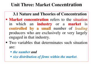
The Phillips Curve, introduced by economist A.W. Phillips in 1958, initially showed an inverse relationship between unemployment rate (u%) and inflation rate (tt%). This led policymakers to consider a trade-off between reducing unemployment and increasing inflation. However, the concept faced challenges during the 1970s with stagflation, leading to the development of the Long-Run Phillips Curve theory by Friedman and Phelps. The natural rate of unemployment plays a crucial role in these models, reflecting the equilibrium rate where real wages balance labor supply and demand. Structural changes in the economy can shift the Long-Run Phillips Curve, emphasizing the need for supply-side policies to address unemployment shifts.

• Phillips Curve
• Monetary Policy
• Unemployment
• Inflation
• Stagflation

anjam Follow

Uploaded on Sep 14, 2024 | 0 Views

Download Presentation

Please find below an Image/Link to download the presentation.

The content on the website is provided AS IS for your information and personal use only. It may not be sold, licensed, or shared on other websites without obtaining consent from the author. Download presentation by click this link. If you encounter any issues during the download, it is possible that the publisher has removed the file from their server.

Presentation Transcript

1. AP Macro Phillips Curve, Monetary Policy

2. The Phillips Curve (hypothetical example) tt% . . . . 4% . . 2% . PC 5% 7% u% Note: Inflation Expectations are held constant

3. The Phillips Curve In a 1958 paper, New Zealand born economist, A.W. Phillips published the results of his research on the historical relationship between the unemployment rate (u%) and the rate of inflation (tt%) in Great Britain. His research indicated a stable inverse relationship between the u% and the tt%. As u% , tt% ; and as u% , tt% . The implication of this relationship was that policy makers could exploit the trade-off and reduce u% at the cost of increased tt%.

4. Trouble for the Phillips Curve In the 1970 s the U.S. experienced concurrent high u% & tt%, = stagflation. 1976 American Nobel Prize economist Milton Friedman saw stagflation as disproof of the stable PC. Instead of a trade-off between u% & tt%, Friedman and 2006 Nobel Prize recipient Edmund Phelps believed that Un was independent of the tt%. This independent relationship is now referred to as the Long-Run Phillips Curve.

5. 1970s Phillips Curve % . . . . . . . . .. . 4% . . . 2% . PC 5% 7% u%

6. The Long-Run Phillips Curve % LRPC un% u% Note: Natural rate of unemployment is held constant

7. Un defined The natural rate of unemployment (NRU) is defined as the equilibrium rate of unemployment i.e. the rate of unemployment where real wages have found their free market level It is where the aggregate supply of labor is in balance with the aggregate demand for labor. At the natural rate, all those wanting to work at the prevailing real wage rate have found employment and there is no involuntary unemployment There remains some voluntary unemployment as some people remain out of a job searching for work offering higher real wages or better conditions.

8. The Long-Run Phillips Curve (LRPC) b/c the LRPC exists at the un, structural changes in the economy that affect un will also cause the LRPC to shift. In order to reduce the Un, structural policies must be directed towards an economy's supply side. Increases in un will shift LRPC Decreases in un will shift LRPC

9. LRPC Inflation rate 4% 2% SRPC (assumes 4 % expected inflation at each UR) SRPC (assumes 2% expected inflation at each UR) Natural rate of unemployment Unemployment rate Phillips Curve LR and SR

10. Summary There is a short-run trade off between u% & %. This is referred to as a short-run Phillips Curve (SRPC) In the long-run, no trade-off exists between u% & %. This is referred to as the long-run Phillips Curve (LRPC) The LRPC exists at the natural rate of unemployment (un). un .: LRPC un .: LRPC C, IG, G, and/or XN = AD = along SRPC AD .: GDPR & PL .: u% & % .: up/left along SRPC AD .: GDPR & PL .: u% & % .: down/right along SRPC Inflationary Expectations, Input Prices, Productivity, Business Taxes and/or Regulation = SRAS = SRPC SRAS .: GDPR & PL .: u% & % .: SRPC SRAS .: GDPR & PL .: u% & % .: SRPC

11. Reconciling the LRPC and SRPC In the long-run, the inflation rate at B ( 1%) becomes the new expected inflation rate ( 1^%), and the economy returns to the natural rate of unemployment (point C). LRPC tt% B C tt1% Assume that either the government or the central bank enacts an expansionary policy to reduce the unemployment rate below its natural rate at point A. A tt % In the short-run, assuming the policy is successful, inflation occurs and unemployment decreases as the economy moves from A to B. SRPC (tt1^ %) SRPC (tt^ %) u% uN% u%

12. Reconciling the LRPC and SRPC In the long-run, the inflation rate at B ( 1%) becomes the new expected inflation rate ( 1^%), and the economy, once again, returns to the natural rate of unemployment (point C). LRPC % A % Now assume that either the government or the central bank enacts a Contractionary policy to reduce inflation from it s current rate at point A C B 1% SRPC ( ^ %) SRPC ( 1^ %) u% uN% u% In the short-run, assuming the policy is successful, disinflation occurs and unemployment increases as the economy moves from A to B.

13. Relating Phillips Curve to AS/AD Changes in the AS/AD model can also be seen in the Phillips Curves An easy way to understand how changes in the AS/AD model affect the Phillips Curve is to think of the two sets of graphs as mirror images. NOTE: The 2 models are not equivalent. The AS/AD model is static, but the Phillips Curve includes change over time. Whereas AS/AD shows one time changes in the price-level as inflation or deflation, The Phillips curve illustrates continuous change in the price-level as either increased inflation or disinflation.

14. Movements along the SRPC

15. Shifts of the SRPC Expected TT: If TT goes up shift up. If TT goes down shift down SRAS increases = shift SRPC right SRAS decreases = shift SRPC left

16. Shifts of the LRPC

17. Increase in AD = Up/left movement along SRPC % PL LRAS . . SRAS SRPC . . P1 1 P AD1 AD un u u% Y YF GDPR C , IG , G and/or XN .: AD .: GDPR & PL .: u% & % .: up/left along SRPC

18. Decrease in AD = Down/right along SRPC LRAS PL % . . SRAS SRPC . . P P1 1 AD AD1 YF Y GDPR u un u% C , IG , G and/or XN .: AD .: GDPR & PL .: u% & % .: down/right along SRPC

19. SRAS = SRPC SRAS SRPC PL % LRPC LRAS . . SRAS1 SRPC1 . . P 1 P1 AD un u u% Y YF GDPR Inflationary Expectations , Input Prices , Productivity , Business Taxes , and/or Deregulation .: SRAS .: GDPR & PL .: u% & % .: SRPC (Disinflation)

20. SRAS = SRPC SRAS1 SRPC1 % PL LRAS LRPC SRAS SRPC . . . . P1 1 P AD Y1 YF GDPR un u1 u% Inflationary Expectations , Input Prices , Productivity , Business Taxes , and/or Increased Regulation .: SRAS .: GDPR & PL .: u% & % .: SRPC (Stagflation)

21. Phillips Curve Review SRAS increases = shift SRPC right SRAS decreases = shift SRPC left AD increases = movement up and left AD decreases = movement down and right Increases in un will shift LRPC Decreases in un will shift LRPC

22. MS NIR MS affected by actions of the Federal Reserve MD i1 Transaction demand determined by GDP Asset demand determined by NIR MD Q1 Q Money Market