Understanding Market Structures: Perfect Competition Overview

Slide Note

This session delves into analyzing different market structures, focusing on perfect competition. It defines market structure, explores key characteristics influencing buyer-seller interactions, and outlines the model of perfect competition. The session discusses how market classification is based on factors like the number of buyers/sellers, product standardization, and barriers to entry. Essential topics covered include the nature of perfect competition, behavior of firms in competitive markets, demand and supply curves, and recommended reading materials.

ama_ruy Follow

Uploaded on Sep 21, 2024 | 0 Views

Download Presentation

Please find below an Image/Link to download the presentation.

The content on the website is provided AS IS for your information and personal use only. It may not be sold, licensed, or shared on other websites without obtaining consent from the author. Download presentation by click this link. If you encounter any issues during the download, it is possible that the publisher has removed the file from their server.

E N D

Presentation Transcript

Lecturer: Dr. (Mrs.) Nkechi S. Owoo, Department of Economics Contact Information: nowoo@ug.edu.gh College of Education School of Continuing and Distance Education 2014/2015 2016/2017

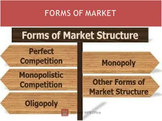
Session Overview This session is the first of three that analyze different market structures. Market structure is a way of describing those characteristics of a market that influence the behavior of buyers and sellers when they come together to trade. To determine market structure, we must ask how many buyers and sellers are in the market, whether the product is standardized, and whether there are barriers to entry. The answers to these questions help to classify a market into one of four basic types: perfect competition, monopoly, monopolistic competition, or oligopoly. This session discusses the model of perfect competition. Slide 2

Session Outline The key topics to be covered in the session are as follows: What is Perfect Competition? The Perfectly Competitive Firm The Competitive Firms Demand Curve The Competitive Firms Supply Curve Slide 3

Reading List Hall and Lieberman Chapter 8, pp:219- 227 Slide 4

Topic One WHAT IS PERFECT COMPETITION? Slide 5

6 Firms in Competitive Markets: Introduction Market Structure This refers to the x tics of a market that influence how trading takes place How do we determine structure of a particular market? How many buyers and sellers are in the market? Is each seller offering a standardized product? Are there any barriers to entry or exit? Is there perfect knowledge about products? There are four main classifications of markets Perfect Competition Monopoly Monopolistic competition Oligopoly For this semester, we shall discuss the first 2 market structures.

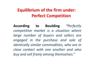
7 Perfect Competition Many buyers and sellers This condition is important so that no individual decision maker can significantly affect the price of the product Consider the market for maize vs. athletic shoes (Nike, Adidas, New Balance) Maize is a good example of a perfectly competitive market Standardized product buyers do not perceive differences between the products e.g. beans. The conditions of many buyers and sellers, and the presence of a standardized product imply that no single buyer or seller has any control over price Would a seller charge more than the going market price? No, because buyers can buy the same product from another seller Would a buyer demand a lower price? No, because sellers can sell at the given price to other consumers Therefore, in a perfectly competitive market, buyers and sellers are price takers.

8 Perfect Competition Sellers can easily enter/exit the market Entry: There are no significant barriers to discourage new entrants Same terms of entry for all firms Can you think of some potential barriers to entry? Large capital requirements, taxation, consumer base, etc Exit: Any firm can enter and exit the market at any time. A firm should be able to sell of equipment and exit market if making losses in the long run Can you think of some potential barriers to exit? Severance pay to workers, inability to sell of specialized machinery, etc This condition is important for long-run outcomes in competitive markets, which we will discuss in part 3

9 Perfect Competition Presence of well-informed buyers and sellers E.g. the Market for maize is a good example Not all markets satisfy this condition, however Consumers who purchase China fabrics or buy used items e.g. cars, do not have perfect knowledge of the goods being purchased.

10 The Perfectly Competitive Firm A market is collection of individual buyers and sellers In PC markets, individual buyers and sellers and overall body (market) affect each other through feedback mechanisms Therefore, must understand how firm works ..and the competitive market in which it operates

11 The Competitive Firm s Demand Curve The demand curve facing the perfectly competitive firm is horizontal perfectly elastic - at the market price i.e. No matter how much firm produces, will sell at the same price Why? Output is standardized If firm charges even a little above competitors, will lose all customers Firm is a tiny producer in overall market Firm can increase production without lowering price Price taker The price of its output is given Decision The firm s main decision is therefore to determine how much output to produce and sell

12 Demand Curves for the Firm and the Industry The demand curves facing the firm is different from the industry demand curve. A perfectly competitive firm s demand schedule is perfectly elastic even though the demand curve for the market is downward sloping.

13 The Competitive Firm s Demand Curve vs. The Competitive Industry Demand Curve The Competitive Industry and Firm 1. The intersection of the market supply and the market demand curve 3. The typical firm can sell all it wants at the market price Market Firm Price Price S $400 $400 Demand Curve Facing the Firm D Output Output 2. determines the equilibrium market price 4. so it faces a horizontal demand curve.

14 The Revenue of a Competitive Firm In the perfect competitive market structure, we assume that firms try to maximize profits Illustration

15 Cost and Revenue Data for a Competitive Firm (Market for Maize) Marginal Revenue Marginal Cost Output (bags of maize) Price per bag Total Revenue (P x Q) Average Revenue (TR/ Q) Total Cost Profit 0 400 0 550 -550 1 400 400 400 400 1000 450 -600 2 400 800 400 400 1200 200 -400 3 400 1200 400 400 1250 50 -50 4 400 1600 400 400 1350 100 250 5 400 2000 400 400 1500 150 500 6 400 2400 400 400 1750 250 650 7 400 2800 400 400 2100 350 700 8 400 3200 400 400 2550 450 650 9 400 3600 400 400 3100 550 500 10 400 4000 400 400 3750 650 250

16 Profit maximization Profits= TR- TC Firm produces at point that maximizes profits as much as possible What then, is the profit-maximizing output level?

17 Cost and Revenue Data for a Competitive Firm Output Price per ounce Total Revenue Marginal Revenue Total Cost Marginal Cost Profit 0 400 0 550 -550 1 400 400 400 1000 450 -600 2 400 800 400 1200 200 -400 3 400 1200 400 1250 50 -50 4 400 1600 400 1350 100 250 5 400 2000 400 1500 150 500 6 400 2400 400 1750 250 650 7 400 2800 400 2100 350 700 8 400 3200 400 2550 450 650 9 400 3600 400 3100 550 500 10 400 4000 400 3750 650 250

18 Profit Maximization Profit Maximization in Perfect Competition (a) TR-TC Ghc TR TC 2,800 Profit = TR-TC Maximum Profit per Day = 700 2,100 550 Slope = 400 1 2 3 4 5 6 7 8 9 10 Bags of Maize per Day

19 Profit maximization Another way to look at profit-maximizing output level MR- MC approach When MR > MC, increases in output increase profits When MC > MR, increases in output reduces profits

20 Cost and Revenue Data for a Competitive Firm Output Price per ounce Total Revenue Marginal Revenue Total Cost Marginal Cost Profit 0 400 0 550 -550 1 400 400 400 1000 450 -600 2 400 800 400 1200 200 -400 3 400 1200 400 1250 50 -50 4 400 1600 400 1350 100 250 5 400 2000 400 1500 150 500 6 400 2400 400 1750 250 650 7 400 2800 400 2100 350 700 8 400 3200 400 2500 450 650 9 400 3600 400 3100 550 500 10 400 4000 400 3750 650 250

21 Profit Maximization Profit Maximization in Perfect Competition (b) MR=MC Dollars Profit maximization MR=MC MC B A $400 d = MR 1 2 3 4 5 6 7 8 9 10 Bags of Maize per Day Rules for Profit Maximization: 1. If MR> MC, firm should increase output 2. If MC> MR, firm should decrease output 3. When MC= MR, profits are maximized

22 Profit Maximization MC- MR approach Produce where MR= MC, and MC crosses MR from below!

23 The Firm s Short-Run Supply Curve The firm takes the market price as given decides how much output to produce at that price Profit-maximizing output level: P=MC (=MR) As price of output changes, firm will slide along its MC curve in deciding how much to produce Recall a firm s cost curves? (AVC, ATV, AFC, MC) Graphical Illustration

24 Recap: Standard Cost Curves Ghc MC 4 3 AFC ATC 2 AVC 1 30 90 130 160 196 0 Units of Output

25 The Firm s Short-Run Supply Curve Short-Run Supply Under Perfect Competition (a) (b) Price per Bushel Dollars ATC Firm's Supply Curve MC $3.50 $3.50 d1=MR1 2.50 2.50 d2=MR2 d3=MR3 2.00 2.00 AVC 1.00 1.00 d4=MR4 d5=MR5 0.50 0.50 Bushels per Year Bushels per Year 1,000 4,000 7,000 2,000 4,000 7,000 2,000 5,000 5,000

26 The Firm s Short-Run Supply Curve As the price of output changes, firm will slide along MC curve in deciding how much to produce But what if firm is suffering a loss A loss large enough to justify shutting down?

27 The Firm s Short-Run Supply Curve What if P= Ghc2? (a) (b) Price Ghc ATC Firm's Supply Curve MC 3.50 3.50 d1=MR1 2.50 2.50 d2=MR2 d3=MR3 2.00 2.00 AVC 1.00 1.00 d4=MR4 d5=MR5 0.50 0.50 Output Output 1,000 4,000 7,000 2,000 4,000 7,000 2,000 5,000 5,000

28 The Firm s Short-Run Supply Curve What if P= Ghc0.50? (a) (b) Price Ghc ATC Firm's Supply Curve MC 3.50 3.50 d1=MR1 2.50 2.50 d2=MR2 d3=MR3 2.00 2.00 AVC 1.00 1.00 d4=MR4 d5=MR5 0.50 0.50 Output Output 1,000 4,000 7,000 2,000 4,000 7,000 2,000 5,000 5,000

29 The Firm s Short-Run Supply Curve What if P= Ghc1? (a) (b) Price Ghc ATC Firm's Supply Curve MC 3.50 3.50 d1=MR1 2.50 2.50 d2=MR2 d3=MR3 2.00 2.00 AVC 1.00 1.00 d4=MR4 d5=MR5 0.50 0.50 Output Output 1,000 4,000 7,000 2,000 4,000 7,000 2,000 5,000 5,000

30 The Shutdown Price Price at which a firm is indifferent between producing and shutting down If P>AVC produce If P<AVC shut down Firm s supply curve Is its MC curve for all prices above AVC, and a vertical line at zero units for all prices below AVC.

31 The Shutdown Point The firm will shut down if it cannot cover average variable costs. A firm should continue to produce as long as price is greater than average variable cost. i.e. P> AVC Once price falls below that point it makes sense to shut down temporarily and save the variable costs. Consider the case of Basement on campus

32 The Shutdown Point The shutdown point is the point at which the firm will gain more by shutting down than it will by staying in business. As long as total revenue is more than total variable cost, temporarily producing at a loss is the firm s best strategy since it is taking less of a loss than it would by shutting down.